Next: 5.3.4 Transformation of a Up: 5.3 Solutions of a Previous: 5.3.2 Transfer matrix for
 (see Eq. (5.35)) of the non-homogeneous differential equation
 is the normed solution of the corresponding homogeneous
differential equation.
To be more precise,
is the normed solution of the corresponding homogeneous
differential equation.
To be more precise,
 are
are
For the particular solution
 at a constant load
  , we
evaluate the following integral:
, we
evaluate the following integral:
 , the particular solution is
 , this particular solution will be in agreement with those examined in [Krä91a], [Krä91b], and [Bor79b].
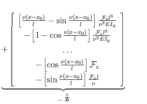
In case of the point load
 , the particular solution is
The general solution of the non-homogeneous differential equation (5.65)
is the sum of the solution of the homogeneous differential equation (5.48) (Sign Convention 2) and
the particular solutions of Eqs. (5.75), (5.76), and (1.36).
Let us take the derivatives of the displacement of Eq. (5.77) and apply these to the governing differential equations (5.3), (5.27), and (5.18).
We get the following beam governing equations
in transfer matrix form (for the compressive axial force, Sign Convention 2):
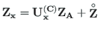
Employing a symbolic matrix notation, the above equations
can be written as
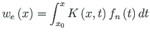
Consider next the finding of the particular solution with the Cauchy formula of Eq. (5.66)
where the normed fundamental set of solutions for the tensile axial force of Eq. (5.43) is
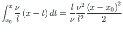
at the constant load (for the tensile axial force),
we evaluate the following integral:
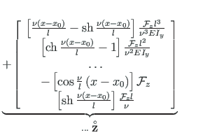
 , the particular solution is
The general solution of the non-homogeneous differential equation (5.65) in case of the tensile axial force is the sum of the solution of the homogeneous differential equation (5.49) (Sign Convention 2) and
the particular solutions of Eqs. (5.84), (5.85), and (1.36).
Let us take the derivatives of the displacement of Eq. (5.86) and apply these to the governing differential equations (5.3), (5.27), and (5.18).
We get the beam governing equations (5.87) in transfer matrix form (for the tensile axial force, Sign Convention 2):
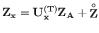
In a symbolic matrix notation, these equations
can be written as
Equations (5.78) and (5.87) should be complemented with the normal force  and the displacement
  .
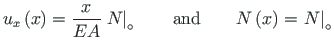
The axial deformation of a frame element
.
The axial deformation of a frame element
 - normal force at the beginning of the element,
 - axial stiffness of the element.
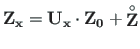
The symbolic matrix transfer equation with the normal force and Sign Convention 2 is
 is that given in Eq. (5.62) and the vector of applied loads,
 , is shown in Table C.5;
 is that given in Eq. (5.64) and the vector of applied loads,
 , is shown in Table C.6.
The transfer matrices
 and
and
 [Krä91b] can be computed using the
GNU Octave function ylfmII.m
(p.
[Krä91b] can be computed using the
GNU Octave function ylfmII.m
(p. ![]() ).
).
The loading vectors
 (5.92) and
 (5.93) for the constant load
  in case of the compression and tension force
  , respectively, are:
The loading vectors
 (5.94) and
 (5.95) for the point load
 in case of the compression and tension force
  ,
respectively, are:
,
respectively, are:
![$\displaystyle \left[{w}^{\prime\prime}\right]^{\prime\prime} {\mp} {\vert}
\fra...
...ght)/{EI_{y}} + \mathcal{M}_{x}{\delta}^{\prime}\left(t - x_{0}\right)/{EI_{y}}$](img617.png)


![$\displaystyle w_{4}\left(x - t\right) = - \left(\frac{l}{\nu}
\right)^{3}\left[...
...\left(x - t\right)\right) -
\left(\frac{\nu}{l}\left(x - t\right)\right)\right]$](img890xx.png)


![$\displaystyle w_{3}\left(x - t\right) = - \left(\frac{l}{\nu}\right)^{2}\left[\cos\left(\frac{\nu}{l}\left(x - t\right)\right) - 1\right]$](img893xx.png)


![$\displaystyle w_{e}\left(x\right) = - \left(\frac{l}{\nu}\right)^{3}\frac{q_{z}...
...eft(x - t\right)\right) -
\left(\frac{\nu}{l}\left(x - t\right)\right)\right]dt$](img623.png)
![$\displaystyle \int_{x_{0}}^{x}\sin\left(\frac{\nu}{l}\left(x - t\right)\right)d...
...ac{l}{\nu}\left[1 - \cos\left(\frac{\nu}{l}\left(x -
x_{0}\right)\right)\right]$](img624.png)
![$\displaystyle w_{e}\left(x\right) = \frac{1}{2\nu^{4}}\left[\frac{\nu^{2}\left(...
... \cos\frac{\nu}{l}\left(x -
x_{0}\right)\right)\right]\frac{q_{z}l^{4}}{EI_{y}}$](img626.png)
![$\displaystyle w_{e}\left(x\right) = -\left(\frac{l}{\nu}\right)^{2}\frac{\mathc...
..._{0}}^{x} \left[\cos\left(\frac{\nu}{l}\left(x - t\right)\right) - 1\right]dt =$](img628.png)
![$\displaystyle = - \left[\sin\left(\frac{\nu}{l}\left(x - x_{0}\right)\right) -
...
...eft(x - x_{0}\right)\right)\right]
\frac{\mathcal{F}_{z}l^{3}}{{\nu}^{3}EI_{y}}$](img629.png)
![$\displaystyle \left.\frac{Q_{z}}{EI_{y}}\right\vert _{\circ}\left(\frac{l}{\nu}...
...\left(
\frac{l}{\nu}\right)^{2}\left[\cos\left(\frac{\nu}{l}x\right) - 1\right]$](img631.png)
![$\displaystyle \frac{1}{2\nu^{4}}\left[\frac{\nu^{2}\left(x -
x_{0}\right)^{2}}{...
... \cos\frac{\nu\left(x -
x_{0}\right)}{l}\right)\right]\frac{q_{z}l^{4}}{EI_{y}}$](img632.png)
![$\displaystyle \left[\left(\frac{\nu}{l}\left(x - x_{0}\right)\right) -
\sin\lef...
...eft(x - x_{0}\right)\right)\right]
\frac{\mathcal{F}_{z}l^{3}}{{\nu}^{3}EI_{y}}$](img633.png)
![$\displaystyle \underbrace{\left[\begin{array}{c}
w_{x} \\
\varphi_{x} \\
\ldo...
...\varphi_{A} \\
\ldots \\
Q_{A} \\
M_{A}
\end{array}\right]}_{\mathbf{Z_{A}}}$](img634.png)
![$\displaystyle %\hspace*{30pt}\nonumber \\ %%\normalsize
{\normalsize { \underb...
...2}}
\end{array} \right]}_{\mathbf{\stackrel{\rm\circ}{Z}} \hspace*{3pt} ...} }}$](img635.png)


![$\displaystyle w_{4}\left(x - t\right) = \left(\frac{l}{\nu}\right)^{3}\left[ \m...
...\left(x - t\right)\right) -
\left(\frac{\nu}{l}\left(x - t\right)\right)\right]$](img638.png)


![$\displaystyle w_{3}\left(x - t\right) = \left(\frac{l}{\nu}\right)^{2}\left[ \mathrm{ch}\left(\frac{\nu}{l}\left(x - t\right)\right) -
1\right]$](img639.png)


![$\displaystyle w_{e}\left(x\right) = \left(\frac{l}{\nu}\right)^{3}\frac{q_{z}}{...
...t(x - t\right)\right) -
\left(\frac{\nu}{l}\left(x - t\right)\right)\right]dt =$](img640.png)
![$\displaystyle - \left[1 + \frac{1}{2}\left(\frac{\nu \left(x - x_{0}\right) }{l...
...thrm{ch}\frac{\nu \left(x - x_{0}\right)}{l}\right]\frac{ql^{4}}{\nu^{4}EI_{y}}$](img641.png)
![$\displaystyle w_{e}\left(x\right) = -\left(\frac{l}{\nu}\right)^{2}\frac{\mathc...
...} \left[ \mathrm{ch}\left(\frac{\nu}{l}\left(x - t\right)\right) -
1\right]dt =$](img642.png)
![$\displaystyle = \left[\frac{\nu}{l}\left(x - x_{0}\right) -
\mathrm{sh}{\,}\fra...
...}{l}\left(x - x_{0}\right)
\right]
\frac{\mathcal{F}_{z}l^{3}}{{\nu}^{3}EI_{y}}$](img643.png)


![$\displaystyle \left.\frac{Q_{z}}{EI_{y}}\right\vert _{\circ}\left(\frac{l}{\nu}...
...frac{l}{\nu}\right)^{2}\left[ \mathrm{ch}\left(\frac{\nu}{l}x\right) - 1\right]$](img644.png)

![$\displaystyle \left[1 + \frac{1}{2}\left(\frac{\nu \left(x - x_{0}\right) }{l}\...
...thrm{ch}\frac{\nu \left(x - x_{0}\right)}{l}\right]\frac{ql^{4}}{\nu^{4}EI_{y}}$](img645.png)

![$\displaystyle \left[\frac{\nu}{l}\left(x - x_{0}\right) -
\mathrm{sh}{\,}\frac{\nu}{l}\left(x - x_{0}\right)
\right]
\frac{\mathcal{F}_{z}l^{3}}{{\nu}^{3}EI_{y}}$](img646.png)
![$\displaystyle \underbrace{\left[\begin{array}{c}
w_{x} \\
\varphi_{x} \\
\ldo...
...\varphi_{A} \\
\ldots \\
Q_{A} \\
M_{A}
\end{array}\right]}_{\mathbf{Z_{A}}}$](img945xx.png)
![$\displaystyle %\hspace*{30pt}\nonumber \\ %%\normalsize
{\normalsize { \underb...
...}}
\end{array} \right]} _{\mathbf{\stackrel{\rm\circ}{Z}} \hspace*{3pt} ...} }}$](img647.png)
![$\displaystyle \mathbf{Z_{x}} = \left[ \begin{array}{c}
u \\
w \\
\varphi_{y} ...
...
w \\
\varphi_{y} \\
N_{x} \\
Q_{z} \\
M_{y}
\end{array} \right]_{0}
\quad$](img653.png)
![$\displaystyle \mathbf{\stackrel{\rm\circ}{ {Z}}}{ }^{+} =
\left[\begin{array}{c...
...- x_{0}\right)}{l} \right) - 1 \right]\frac{ql^{2}}{\nu^{2}}
\end{array}\right]$](img662.png)
![$\displaystyle \mathbf{\stackrel{\rm\circ}{ {Z}}}{ }^{-} =
\left[\begin{array}{c...
...( x - x_{0}\right)}{l} \right) \right]\frac{ql^{2}}{\nu^{2}}
\end{array}\right]$](img663.png)
![$\displaystyle \mathbf{\stackrel{\rm\circ}{ {Z}}}{ }^{+} =
\left[\begin{array}{c...
... x_{0}\right)}{l}\right) \right]\frac{\mathcal{F}_{z}l}{\nu}
\end{array}\right]$](img664.png)
![$\displaystyle \mathbf{\stackrel{\rm\circ}{{Z}}}{ }^{-} =
\left[\begin{array}{c}...
...frac{\left(x - x_{0}\right)}{l}\right) \right]\frac{Fl}{\nu}
\end{array}\right]$](img665.png)