5.3.4 Transformation of a transfer matrix

Let $X$, $Z$ be the global coordinate system (see Fig. 5.5), $x$, $z$ the local (initial) coordinate system, and $\xi$, $\eta$ the current coordinate system [Yaw09].

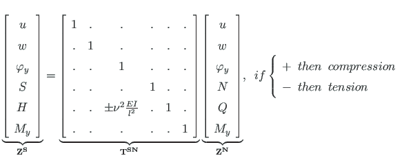
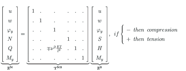
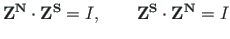
We have derived the transfer matrix $\mathbf{U_{x}}$ from Eq. (5.90) for the normal force N and shear force $Q$ shown in Fig. 5.1. These forces (N, $Q$) we bind with the current coordinate system ($\xi$, $\eta$).

Figure 5.5: Axial and normal forces

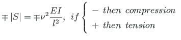
The axial force $S$ and transverse shear force $H$ are described in the initial (local) coordinate system ($x$, $z$). In the global coordinate system ($X$, $Z$), the joint equilibrium equations are written.

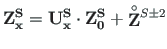
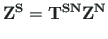
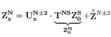
We now consider a symbolic matrix transfer equation at the axial force S and Sign Convention 2:

$$\mathbf{Z_{x}^{S}} = \mathbf{U^{S}_{x}\cdot Z_{0}^{S}} + \mathbf{{\stackrel{\rm\circ}{Z}}}{ }^{S\pm 2}$$ (5.96)

where

$$\mathbf{Z_{x}^{S}} = \left[ \begin{array}{c} u \\ w \\ \varphi_... ... w \\ \varphi_{y} \\ S_{x} \\ H_{z} \\ M_{y} \end{array} \right]_{0} \quad$$ (5.97)

From Eq. (5.4)

$$N + \underbrace{Q\varphi}_{{\ll} N} = S_{x} {\cong} N$$

$$N = \mp \left\vert S\right\vert = \mp {\nu}^{2}\frac{EI}{l^{2}}, \ens... ...hen \enspace compression \\ +\enspace then \enspace tension \end{array}\right.$$ (5.98)

and the relationship between the forces referred to a deformed and undeformed axis can be rewritten [Krä91b] in the form of Eq. (5.4):

$$\left[ \begin{array}{c} H \end{array}\right] = \left[ \begin{arra... ...nspace compression \\ -\enspace then \enspace tension \end{array}\right. \quad$$ (5.99)

Due to the orthogonality of Eq. (A.27), we can write from the inverse of the matrix of Eq. (5.4)

$$\left[ \begin{array}{c} Q \end{array}\right] = \left[ \begin{arra... ...nspace compression \\ +\enspace then \enspace tension \end{array}\right. \quad$$ (5.100)

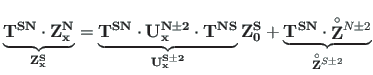
In order to change variables $N$, $Q$ to $S$, $H$, we will need the transformation relations of Eq. (5.101) [Krä91b]:

$$\underbrace{\left[ \begin{array}{c} u \\ w \\ \varphi_{y} \\ S... ...nspace compression \\ -\enspace then \enspace tension \end{array}\right. \quad$$ (5.101)

or

$$\mathbf{{Z}^{S}} = \mathbf{{T}^{SN}}\mathbf{Z^{N}}$$ (5.102)

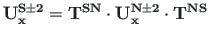
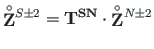
To compute the transformation matrix $\mathbf{{T}^{SN}}$, the GNU Octave function ytransf.m (p. ) can be used.

We will make the inverse change of variables $S$, $H$ to $N$, $Q$ with the equations

$$\underbrace{\left[ \begin{array}{c} u \\ w \\ \varphi_{y} \\ N... ...nspace compression \\ +\enspace then \enspace tension \end{array}\right. \quad$$ (5.103)

or

$${\mathbf{{Z}^{N}}} = {\mathbf{{T}^{NS}}}{\mathbf{{Z}^{S}}}$$ (5.104)

Here, the transformation matrix $\mathbf{{T}^{NS}}$ can be computed using the GNU Octave function ytransfp.m (p. ).

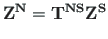
The matrix ${\mathbf{{Z}^{N}}}$ has the inverse matrix ${\mathbf{{Z}^{S}}}$, i.e

$$\mathbf{{Z}^{N}}\cdot \mathbf{{Z}^{S}} = I, \qquad \mathbf{{Z}^{S}}\cdot \mathbf{{Z}^{N}} = I$$ (5.105)

We rewrite Eq. (5.90) in the form

$$\mathbf{Z^{N}_{x}} = \mathbf{U^{N\pm 2}_{x}}\cdot \underbrace{{\m... ...{S}_{0}}}}_{\mathbf{{Z}^{N}_{0}}} + \mathbf{\stackrel{\rm\circ}{Z}}{ }^{N\pm 2}$$ (5.106)

and multiply Eq. (5.106) from left by $\mathbf{{T}^{SN}}$:

$$\underbrace{\mathbf{{T}^{SN}} \cdot\mathbf{Z^{N}_{x}}}_{\mathbf{{... ...krel{\rm\circ}{Z}}{ }^{N\pm 2}}_{\mathbf{{\stackrel{\rm\circ}{Z}}}{ }^{S\pm 2}}$$ (5.107)

When comparing equations (5.96) and (5.107), we show that

$${\mathbf{U^{S\pm 2}_{x}}} = \mathbf{{T}^{SN}} \cdot\mathbf{U^{N\pm 2}_{x}}\cdot {\mathbf{{T}^{NS}}}$$ (5.108)

and

$${\mathbf{{\stackrel{\rm\circ}{Z}}}{ }^{S\pm 2}} = \mathbf{{T}^{SN}} \cdot\mathbf{\stackrel{\rm\circ}{Z}}{ }^{N\pm 2}$$ (5.109)

where ${\mathbf{U^{S-2}_{x}}} =$

$$= \left[ \begin{array}{cccccc} 1 & 0 & 0 & -\frac{x}{EA} & 0 & 0 ... ...t) \frac{l}{\nu} & - \cos\left( \frac{\nu x}{l}\right) \end{array}\right] \quad$$ (5.110)

and ${\mathbf{U^{S+2}_{x}}} =$

$$= \left[ \begin{array}{cccccc} 1 & 0 & 0 & -\frac{x}{EA} & 0 & 0 ... ...{l}{\nu} & - \mathrm{ch} \left( \frac{\nu x}{l}\right) \end{array}\right] \quad$$ (5.111)

The transfer matrices (for the axial and transverse shear forces $S$, $H$; Sign Convention 2) $\mathbf{U^{S-2}_{x}}$ of Eq. (5.110) and $\mathbf{U^{S+2}_{x}}$ of Eq. (5.111) can be computed using the GNU Octave function ylfmhvII.m , taking the input argument $baasi0$ equal to 1.0 ($baasi0$ is input for scaling multiplier $i_{0}= EI/l$, see p. ).

If we multiply the loading vectors of Eqs. (5.92) and (5.93) (for the normal and shear forces $N$, $Q$) from left by $\mathbf{{T}^{SN}}$ (see Eq. (5.109)), we get the products of Eqs. (5.112) and (5.113) (for the axial and transverse shear forces $S$, $H$):

$$\mathbf{\stackrel{\rm\circ}{{Z}}}{}^{S-2} = \left[\begin{array}{c... ...- x_{0}\right)}{l} \right) - 1 \right]\frac{ql^{2}}{\nu^{2}} \end{array}\right]$$ (5.112)

$$\mathbf{\stackrel{\rm\circ}{{Z}}}{}^{S+2} = \left[\begin{array}{c... ...( x - x_{0}\right)}{l} \right) \right]\frac{ql^{2}}{\nu^{2}} \end{array}\right]$$ (5.113)

The loading vectors of Eqs. (5.112) and (5.113) can be computed using the GNU Octave function ylqvII.m , taking the input argument $baasi0$ equal to 1.0 ($baasi0$ is input for the scaling multiplier $i_{0}= EI/l$, see p. ).

Multiplying the loading vectors of Eqs. (5.94) and (5.95) (for the normal and shear forces $N$, $Q$) from left by $\mathbf{{T}^{SN}}$ (see Eq. (5.109)), we get the products of Eqs. (5.114) and (5.115) (for the axial and transverse shear forces $S$, $H$):

$$\mathbf{\stackrel{\rm\circ}{{Z}}}{}^{S-2} = \left[\begin{array}{c... ...frac{\left(x - x_{0}\right)}{l}\right) \right]\frac{Fl}{\nu} \end{array}\right]$$ (5.114)

$$\mathbf{\stackrel{\rm\circ}{{Z}}}{}^{S+2} = \left[\begin{array}{c... ...frac{\left(x - x_{0}\right)}{l}\right) \right]\frac{Fl}{\nu} \end{array}\right]$$ (5.115)

The loading vectors of Eqs. (5.114) and (5.115) can be computed using the GNU Octave function ylfhvzII.m (p. ) , taking the input argument $baasi0$ equal to 1.0 ($baasi0$ is input for the scaling multiplier $i_{0}= EI/l$, see p. ).