Next: B. Work and work-energy Up: A. Matrices Previous: A.1.3 Sparse matrix functions
Consider the two right-handed coordinate systems of Fig. A.3, defined by orthogonal unit vectors
 and
and
 .
Let xyz be global coordinates and
.
Let xyz be global coordinates and
 a local coordinate
system.
a local coordinate
system.
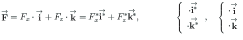
The vector
 in Fig. A.3 can be written as the sum of two vectors along the
coordinate axes
in Fig. A.3 can be written as the sum of two vectors along the
coordinate axes  with magnitude
  ,
,  and along the
coordinate axes
and along the
coordinate axes
 with magnitude
  ,
,  .
.
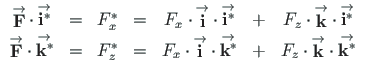
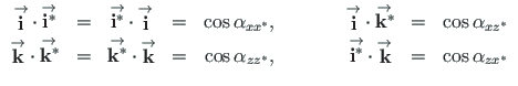
To find the components of the vector
 of Eq. (A.15),
we multiply this equation by
of Eq. (A.15),
we multiply this equation by
 and
and
 . The scalar products are:
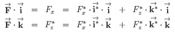
To find the inverse transformation, we multiply Eq. (A.15) by
 and
and
 .
The scalar products are:
.
The scalar products are:
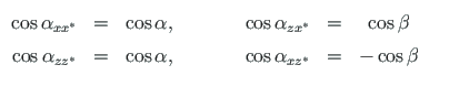
 :
:
 =
=  and
and
 =
=  ( =
( =
 =
=  ).
).
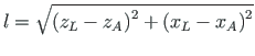
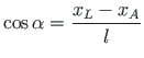
The length l and the direction cosines of an element can be calculated using coordinates  ,
,  of the node at the beginning and coordinates
 ,
,  of the node at the end of the element (Fig. A.4):
We now consider the transformation of the vector
 components
  ,
,  of Eq. (A.15) from the global xy coordinate system to the components
  ,
,  in the
local
in the
local
 coordinate system.
 =
=
 =
=  , we can write the above equation as
The inverse transformation of the vector
 components
  ,
,  of
Eq. (A.15) from the
local
of
Eq. (A.15) from the
local
 coordinate system to the components
  ,
,  of the global xy coordinate system:
 =
=
 =
=  , we can write Eq. (A.25) in the form
Comparing the transformation matrix (A.23) with that of (A.25),
we can see that they are transposed (rows and columns reversed). The multiplication of the matrix (A.23) by a transpose of itself of Eq. (A.25) gives the identity
matrix
![\includegraphics[width=60mm]{joonised/koorteis.eps}](img978.png)
![\includegraphics[width=83mm]{joonised/suunacosen.eps}](img996.png)
![$\displaystyle \left[\begin{array}{c}
F^{\ast}_{x} \\
F^{\ast}_{z}
\end{array} ...
...
\end{array} \right]
\left[\begin{array}{c}
F_{x} \\
F_{z}
\end{array} \right]$](img1001.png)
![$\displaystyle \left[\begin{array}{c}
F^{\ast}_{x} \\
F^{\ast}_{z}
\end{array} ...
...
\end{array} \right]
\left[\begin{array}{c}
F_{x} \\
F_{z}
\end{array} \right]$](img1556xx.png)
![$\displaystyle \left[\begin{array}{c}
F_{x} \\
F_{z}
\end{array} \right] =
\lef...
...right]
\left[\begin{array}{c}
F_{x}^{\ast} \\
F_{z}^{\ast}
\end{array} \right]$](img1002.png)
![$\displaystyle \left[\begin{array}{c}
F_{x} \\
F_{z}
\end{array} \right] =
\lef...
...right]
\left[\begin{array}{c}
F^{\ast}_{x} \\
F^{\ast}_{z}
\end{array} \right]$](img1003.png)
![$\displaystyle \left[\begin{array}{cc}
\cos\alpha & \cos\beta \\
- \cos\beta & ...
...nd{array} \right] =
\left[\begin{array}{cc}
1 & 0 \\
0 & 1
\end{array} \right]$](img1004.png)