Next: 5.3 Solutions of a Up: 5. Second-order structural analysis Previous: 5.1 Introduction
Consider the deformed beam-column element in Fig. 5.1. We must differentiate the
forces in the deformed and undeformed axis of the beam. The axial force  versus normal force
  and
the transverse shear force
and
the transverse shear force  versus shear force
  are depicted in Fig. 5.1.
The beam-column theory uses the Bernoulli5.1-Euler5.2 theory kinematic assumption that the curvature  can be considered equal to the second derivative of the deflected longitudinal axis
 .
.
The relationship of Eq. (A.26) between the forces referred to the deformed and undeformed axis is
 , allows us to conclude that
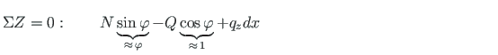
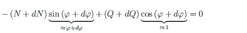
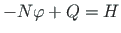
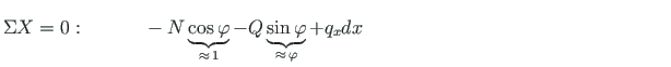
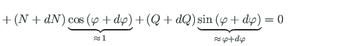
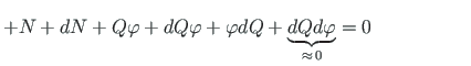
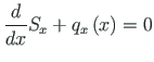
Now we project the forces onto the direction of x-axis:
 is the length of the element.
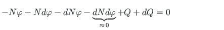
Hence
is the length of the element.
Hence
 , and we rewrite Eq. (5.17):
 is
is
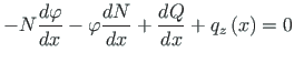
 , and from Eq. (5.16)
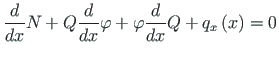
 in the above equation by the expression from Eq. (5.10), and
  by the expression
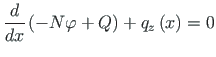
 , we obtain
For a constant axial force  and a constant
  we obtain
 ) and
the plus sign a compressive axial force (
) and
the plus sign a compressive axial force ( ).
).
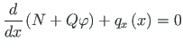
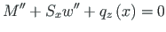
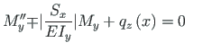
The governing equations (5.28) for the beam-column transverse displacement can
be written as
 , we obtain
 ) and
the plus sign a compressive axial force (
) and
the plus sign a compressive axial force ( ).
).
Equation (5.30) is the differential equation governing the deflection w of
a beam-column member with a constant  , subjected to a constant axial force
at any end restraint.
, subjected to a constant axial force
at any end restraint.
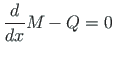
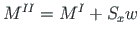
In a second-order analysis, the total deflection w is calculated (see Fig. 5.4).
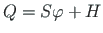
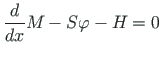
The total bending moment  is the sum of the bending moment
  of
undeformed geometry of the member and the moment Sw (S - axial load, w - displacement) due to the
deformed geometry of the member shown in Fig. 5.4 b. The moment is said to be amplified.
of
undeformed geometry of the member and the moment Sw (S - axial load, w - displacement) due to the
deformed geometry of the member shown in Fig. 5.4 b. The moment is said to be amplified.
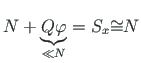
 can be presented with the displacements
  and
and  :
:
![$\left[u^{\prime} + \frac{1}{2}\left(w^{\prime}\right)^{2}\right]$](img557.png) is a large
Kármán5.3-type deflection and
is a large
Kármán5.3-type deflection and  is the axial stiffness.
![\includegraphics[width=105mm]{joonised/pikirist_en.eps}](img502.png)
![$\displaystyle \left[
\begin{array}{c}
S \\
H
\end{array}\right] =
\left[
\begi...
...s\varphi}
\end{array}\right]
\left[
\begin{array}{c}
N \\
Q
\end{array}\right]$](img506.png)
![$\displaystyle \left[
\begin{array}{c}
S \\
H
\end{array}\right] =
\left[
\begi...
...phi & {1}
\end{array}\right]
\left[
\begin{array}{c}
N \\
Q
\end{array}\right]$](img509.png)
![\includegraphics[width=135mm]{joonised/iijarkts.eps}](img510.png)


![$\displaystyle \left[
\begin{array}{c}
N \\
Q
\end{array}\right] =
\left[
\begi...
...phi & {1}
\end{array}\right]
\left[
\begin{array}{c}
S \\
H
\end{array}\right]$](img531.png)
![\includegraphics[width=45mm]{joonised/normkomp.eps}](img533.png)
![\begin{figure}\begin{center}
\begin{overpic}[scale=.6]
{joonised/piki_m.eps}
\p...
...overline{x} -
x\right)dx}_{M^{I}} + Sw$}
\end{overpic}\end{center}
\end{figure}](img550.png)
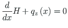
![$\displaystyle \left[EI_{y}{w}^{\prime\prime}\right]^{\prime\prime} {\mp} {\vert}
S_{x}{\vert}{w}^{\prime\prime} - q_{z}\left(x\right) = 0$](img551.png)
![$\displaystyle \left[{w}^{\prime\prime}\right]^{\prime\prime} {\mp} {\vert}
\fra...
...EI_{y}}{\vert}{w}^{\prime\prime} -
\frac{q_{z}\left(x\right)}{EI_{y}} = 0 \quad$](img552.png)
![$\displaystyle S {\approx} {\,} N = - EA\left[u^{\prime} +
\frac{1}{2}\left(w^{\prime}\right)^{2}\right]$](img556.png)