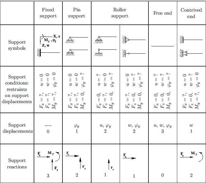
Next: 1.2.2 Basic equations for Up: 1.2 Basic equations for Previous: 1.2 Basic equations for
where
 is the elastic modulus and
  is the area moment of inertia.
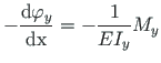
The last formula of Eq. (1.14) is a non-homogeneous differential equation of 4th
order
(
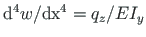 ).
We are looking for the general solution of the
non-homogeneous differential equation in the form
).
We are looking for the general solution of the
non-homogeneous differential equation in the form
 , and
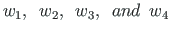
, and
 are the values of the sought-for function at
 ;
;
 are a normed fundamental set of solutions to
the associated homogeneous differential equation;
are a normed fundamental set of solutions to
the associated homogeneous differential equation;
 is the particular solution of the non-homogeneous differential equation.
Next we consider a set for fundamental solutions for
the associated homogeneous differential equation:
The Wronskian1.1  of this set of solutions

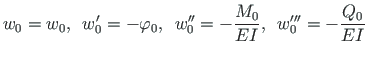
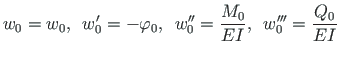
By Sign Convention 1, the initial parameters of
Eq. (1.15) are
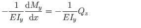
Substituting Eqs. (1.16) and (1.19) into Eq. (1.15), we
get the solution for the homogeneous differential equation
(Sign Convention 1):
The general non-homogeneous differential equation
of the Euler-Bernoulli beam subjected to an external load and equivalent generalized loads is
 is the equivalent distributed force
  of a concentrated force of magnitude
 ,
,
 is the equivalent distributed force
  of a concentrated moment of magnitude
 ,
,
 is the Dirac delta function.
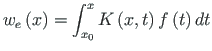
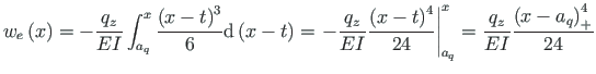
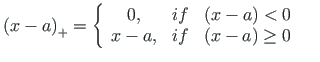
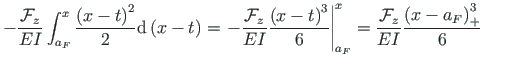
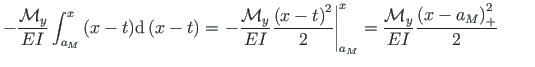
The particular solution
of Eq. (1.15) we are looking for is given by the Cauchy formula
 is
is
The particular solution
 at a constant load
 is the Heaviside step function:
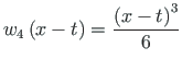
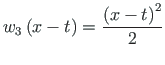
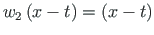
In case of the point load
 and moment
 , the functions
,
, the functions
,
 in the Cauchy formula (1.24) are respectively
The particular solution
 in case of the point load
 and moment
 is respectively
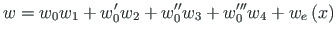
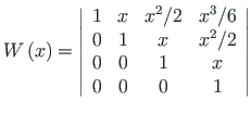
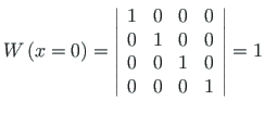
The general solution of the non-homogeneous differential equation
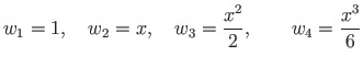
Let us take the derivatives of displacement from Eq. (1.38) and apply those to
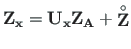
the governing differential equation (1.14). We obtain beam governing equations
with the transfer matrix
 ) from Eq. (1.3) is added to the deformation.
In symbolic matrix notation, the formulae of Eq. (1.39) can be written as
andres
![\includegraphics[width=50mm]{joonised/VardaDiff.eps}](img66.png)


![$\displaystyle w =
\left[\begin{array}{cccc}
1 & - x & - {x^{2}}/{2EI} & -{x^{3}...
...t[\begin{array}{c}
w_{0} \\
\varphi_{0} \\
M_{0} \\
Q_{0}
\end{array}\right]$](img91.png)
![$\displaystyle w =
\left[\begin{array}{cccc}
1 & - x & {x^{2}}/{2EI} & {x^{3}}/{...
...t[\begin{array}{c}
w_{0} \\
\varphi_{0} \\
M_{0} \\
Q_{0}
\end{array}\right]$](img92.png)


![$\displaystyle \underbrace{\left[\begin{array}{c}
w_{x} \\
\varphi_{x} \\
\ldots \\
Q_{x} \\
M_{x}
\end{array}\right]}_{\mathbf{Z_{x}}}$](img127.png)
![$\displaystyle \underbrace{\left[ \begin{array}{ccccc}
1 & - x & \vdots & {x^{3}...
...\varphi_{A} \\
\ldots \\
Q_{A} \\
M_{A}
\end{array}\right]}_{\mathbf{Z_{A}}}$](img128.png)
![$\displaystyle { \large { \underbrace{ \left[\begin{array}{cccccc}
+ & \frac{q_{...
...ray}\right]}_{\mathbf{\stackrel{\rm\circ}{Z}}} }} %
\qquad \qquad \qquad \qquad$](img129.png)