2.2 Compatibility equations of displacements

Consider a system of compatibility equation sets of the joint displacements shown in excerpts 2.1 and 2.2 from the computing diary.

Computing diary excerpt 2.1 ( LaheFrameDFIm.m )  

===============================================================
Element | Displacements | Joint  | Axial, shear, moment hinges
  No    | u_   w_   fi_ | (node) |     0 - hinge 'false' 
        |    indexes    |   No   |     1 - hinge 'true' 
----------------------------------------------------------------
    1      1    2    3      2          0      0      0
    2     19   20   21      2          0      0      0

In excerpt 2.1 from the computing diary, two elements, 1 and 2, at joint node 2 are shown. The displacements of element 1 at node 2 are $Z_{1}$, $Z_{2}$, $Z_{3}$ and the displacements of element 2 at node 2 are $Z_{19}$, $Z_{20}$, $Z_{21}$. The joint at node 2 is rigid (see Fig. 1.12).

We now connect elements 1 and 2, the end displacements of which are

$$\mathbf{v^{\left( 1\right)}_{L}} = \left[\begin{array}{c} u^{\lef... ...\ w^{\left( 2\right)}_{A} \\ \varphi^{\left( j\right)}_{A} \end{array}\right]$$ (2.4)

The compatibility equations at node 2 in global coordinates:

$$\mathbf{T^{\left( 1\right) }_{3\times 3}}\cdot \mathbf{v^{\left( ... ...bf{T^{\left( 2\right) }_{3\times 3}}\cdot \mathbf{v^{\left( 2\right) }_{A}} = 0$$ (2.5)

where the transformation matrices are expressed as

$$\mathbf{T^{\left( 1\right)}_{3\times 3}} = \left[ \begin{array}{c... ...2} & 0 \\ \cos\beta_{2} & \cos\alpha_{2} & 0 \\ 0 & 0 & 1 \end{array} \right]$$ (2.6)

Computing diary excerpt 2.2 ( yspESTframe2LaheWFI.m )  

===============================================================
Element | Displacements | Joint  | Axial, shear, moment hinges
  No    | u_   w_   fi_ | (node) |     0 - hinge 'false' 
        |    indexes    |   No   |     1 - hinge 'true' 
----------------------------------------------------------------    
    2     13   14   15      4          0      0      0
    3     25   26   27      4          0      0      0    
    4     43   44   45      4          0      0      1

In excerpt 2.2 from the computing diary, three elements - 2, 3 and 4 - at joint node 4 are shown. The displacements of element 2 at node 4 are $Z_{13}$, $Z_{14}$, $Z_{15}$, and the displacements of element 4 at node 4 are $Z_{43}$, $Z_{44}$, $Z_{45}$. Element 4 has a bending moment hinge at node 4 (see Fig. 1.12).

Now we connect elements 2 and 4, the end displacements of which are

$$\mathbf{v^{\left( 2\right)}_{L}} = \left[\begin{array}{c} u^{\lef... ...rray}{c} u^{\left( 4\right)}_{A} \\ w^{\left( 4\right)}_{A} \end{array}\right]$$ (2.7)

The compatibility equations for the pair displacements of elements 2 and 4:

$$\mathbf{T^{\left( 2\right) }_{2\times 2}}\cdot \mathbf{v^{\left( ... ...bf{T^{\left( 4\right) }_{2\times 2}}\cdot \mathbf{v^{\left( 4\right) }_{A}} = 0$$ (2.8)

where the transformation matrices (see Eq. (A.25)) have the form

$$\mathbf{T^{\left( 2\right) }_{2\times 2}} = \left[ \begin{array}{... ...ha_{4} & - \cos\beta_{4} \\ \cos\beta_{4} & \cos\alpha_{4} \end{array} \right]$$ (2.9)

There may be a number of displacement pairs of elements: 2-3, 2-4, 3-4, .... The set of pairs 2-3, 2-4, 3-4 is linearly independent. We need a maximal linearly independent subset of the set pairs. A linearly independent set is called maximal if each of its proper superset is linearly dependent [OUD10], [KB95]. Compatibility requirements should be satisfied in the compatibility method, called also the matrix force method. We should note that at rigid joint frames, the multiple hinge is equivalent to n-1 simple hinges (n is the number of members connected in the joint). Here, compatibility equations must be verified to meet all the criteria of transitivity ^2.4. We consider pairs 2-3, 2-4 or pairs 2-3, 3-4, which are linearly independent sets.

Figure 2.1: Transitivity

A relation between element end displacements is transitive whenever a displacement at bar 1 end point is equal to a displacement at bar 2 starting point, and a displacement at bar 3 end point is equal to a displacement at bar 2 starting point. Then the displacement at bar 1 end point is equal to the displacement at bar 3 end point (see Fig. 2.1).

Let us now consider the compatibility of displacements and rotations at the joints.

Displacements at joint A3 (see Fig. 2.2). Here, two elements are connected at a rigid joint.

Figure 2.2: Compatibility at rigid joint A3

$$\left[ \begin{array}{ccc} 0 & 1 & 0 \\ - 1 & 0 & 0 \\ 0 & 0 & 1... ... 2\right)}_{A} \\ \varphi^{\left( 2\right) }_{A} \end{array}\right] = 0 \qquad$$ (2.10)

or

$$\mathbf{T^{\left( 1\right)}_{3\times 3}}\cdot \mathbf{v^{\left( 1... ...\right)}_{3\times 3}}\cdot \mathbf{v^{\left( 2\right) }_{A}} = 0 \vspace*{35pt}$$ (2.11)

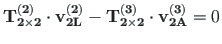
Displacements at joint A2 (see Fig. 2.3). Here, two elements are connected at a hinged joint.

Figure 2.3: Compatibility at hinged joint A2

$$\left[ \begin{array}{cc} 0 & 1 \\ - 1 & 0 \end{array} \right] \l... ...left( 2\right) }_{A} \\ w^{\left( 2\right) }_{A} \end{array}\right] = 0 \qquad$$ (2.12)

         or

$$\mathbf{T^{\left( 1\right)}_{2\times 2}}\cdot \mathbf{v^{\left( 1... ...right)}_{2\times 2}}\cdot \mathbf{v^{\left( 2\right) }_{2A}} = 0 \hspace*{60pt}$$ (2.13)

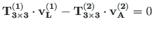
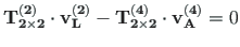
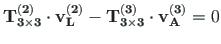
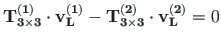
Displacements at joint B3 (see Fig. 2.4). Three elements are connected at a rigid joint. The displacement compatibility for elements 1-2 is given as

$$\left[ \begin{array}{ccc} 1 & 0 & 0 \\ 0 & 1 & 0 \\ 0 & 0 & 1 \... ...2\right) }_{A} \\ \varphi^{\left( 2\right) }_{A} \end{array}\right] = 0 \qquad$$ (2.14)

or

$$\mathbf{T^{\left( 1\right)}_{3\times 3}}\cdot \mathbf{v^{\left( 1... ...hbf{T^{\left( 2\right)}_{3\times 3}}\cdot \mathbf{v^{\left( 2\right) }_{A}} = 0$$ (2.15)

The displacement compatibility for elements 2-3 is given as

Figure 2.4: Compatibility at rigid joint B3

$$\left[ \begin{array}{ccc} 0 & 1 & 0 \\ -1 & 0 & 0 \\ 0 & 0 & 1 ... ... w^{\left( 2\right) }_{L} \\ \varphi^{\left( 2\right) }_{L} \end{array}\right]$$

$$- \left[ \begin{array}{ccc} 1 & 0 & 0 \\ 0 & 1 & 0 \\ 0 & 0 & 1... ...3\right) }_{A} \\ \varphi^{\left( 3\right) }_{A} \end{array}\right] = 0 \qquad$$ (2.16)

or

$$\mathbf{T^{\left( 2\right)}_{3\times 3}}\cdot \mathbf{v^{\left( 2... ...hbf{T^{\left( 3\right)}_{3\times 3}}\cdot \mathbf{v^{\left( 3\right) }_{A}} = 0$$ (2.17)

        

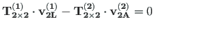
Displacements at joint B32 (see Fig. 2.5). Three elements are gathered together at a joint with rigid and pin connection. Elements 2-3 are connected at the joint by a hinge.

Figure 2.5: Compatibility at rigid & pin joint B32

$$\left[ \begin{array}{ccc} 0 & 1 \\ -1 & 0 \end{array} \right] \l... ...left( 3\right) }_{A} \\ w^{\left( 3\right) }_{A} \end{array}\right] = 0 \qquad$$ (2.18)

or

$$\mathbf{T^{\left( 2\right)}_{2\times 2}}\cdot \mathbf{v^{\left( 2... ...bf{T^{\left( 3\right)}_{2\times 2}}\cdot \mathbf{v^{\left( 3\right) }_{2A}} = 0$$ (2.19)

Elements 1-2 are connected rigidly at the joint. Their displacement compatibility equations are

$$\left[ \begin{array}{ccc} 1 & 0 & 0 \\ 0 & 1 & 0 \\ 0 & 0 & 1 \... ...2\right) }_{L} \\ \varphi^{\left( 2\right) }_{L} \end{array}\right] = 0 \qquad$$ (2.20)

or

$$\mathbf{T^{\left( 1\right)}_{3\times 3}}\cdot \mathbf{v^{\left( 1... ...hbf{T^{\left( 2\right)}_{3\times 3}}\cdot \mathbf{v^{\left( 2\right) }_{L}} = 0$$ (2.21)

Displacements at joint B2 (see Fig. 2.6). Three elements - 1, 2, and 3 - are connected at a pin joint. Elements 1-2 are connected by a hinge.

$$\left[ \begin{array}{ccc} 1 & 0 \\ 0 & 1 \end{array} \right] \le... ...left( 2\right) }_{A} \\ w^{\left( 2\right) }_{A} \end{array}\right] = 0 \qquad$$ (2.22)

or

$$\mathbf{T^{\left( 1\right)}_{2\times 2}}\cdot \mathbf{v^{\left( 1... ...bf{T^{\left( 2\right)}_{2\times 2}}\cdot \mathbf{v^{\left( 2\right) }_{2A}} = 0$$ (2.23)

Figure 2.6: Compatibility at pin joint B2

Elements 2-3 are also connected by a hinge.

$$\left[ \begin{array}{ccc} 0 & 1 \\ -1 & 0 \end{array} \right] \l... ...left( 3\right) }_{A} \\ w^{\left( 3\right) }_{A} \end{array}\right] = 0 \qquad$$ (2.24)

or

$$\mathbf{T^{\left( 2\right)}_{2\times 2}}\cdot \mathbf{v^{\left( 2... ...bf{T^{\left( 3\right)}_{2\times 2}}\cdot \mathbf{v^{\left( 3\right) }_{2A}} = 0$$ (2.25)

        

The transformation matrices $\mathbf{T^{\left( i\right)}_{3\times 3}}$ and $\mathbf{T^{\left( i\right)}_{2\times 2}}$ (in the program as $SpTM3x3$ and $SpTM2x2$) are represented with the functions SpTeisendusMaatriks.m and SpTeisendusMaatriks2x2.m, respectively. The program selects the row index and finds column and element indexes (see excerpts 2.1 and 2.2 from the computing diary). Taking into account the expressions $SpTM3x3m = - SpTM3x3$ and $SpTM2x2m = - SpTM2x2$, the compatibility equations of the displacements at a node can be inserted into Eq. (2.1). The program inserts the transformation matrices with the commands cmd = spA=spInsertBtoA(spA,34,43,SpTM3x3); and cmd = spA=spInsertBtoA(spA,34,25,SpTM3x3m); (see excerpt 2.3).

Computing diary excerpt 2.3 ( spESTframe93LaheWFI.m )  

#====================================================================
----- Sparse matrix instantiation --------  
  spA=sparse(NNK,NNK)  
  
spA =
Compressed Column Sparse (rows = 67, cols = 67, nnz = 0 [0%])

----- Right-hand side of the equations (RHS). --------  
  B=zeros(NNK,1);  

#====================================================================
----- Writing basic equations of a frame ----  
#==================================================================== 

----- Basic equations are inserted into spA  --------  
rows = rows_of_basic_equations: 30
col = cols_of_basic_equations: 60
spA_nnz = non_zero_elements_in_basic_equations: 95
  
#====================================================================
 Compatibility equations of displacements at nodes 
From_row = Compatibility equations begin from row: 31
#====================================================================
Node =  1
Node =  2
cmd = spA=spInsertBtoA(spA,31,19,SpTM3x3);
cmd = spA=spInsertBtoA(spA,31,1,SpTM3x3m);
Node =  3
Node =  4
cmd = spA=spInsertBtoA(spA,34,43,SpTM3x3);
cmd = spA=spInsertBtoA(spA,34,25,SpTM3x3m);
cmd = spA=spInsertBtoA(spA,37,43,SpTM3x3);
cmd = spA=spInsertBtoA(spA,37,13,SpTM3x3m);
Node =  5
Node =  6
cmd = spA=spInsertBtoA(spA,40,55,SpTM3x3);
cmd = spA=spInsertBtoA(spA,40,37,SpTM3x3m);
----- 
spA_rows =  42
spA_cols =  60
spA_nnz = non_zero_elements_in_spA: 129 
--- Compatibility equations of displacements are inserted into spA ---  
compatibility_equations_rows =  12
non_zero_elements_in_compatibility_equations =  34
#====================================================================