Next: IV. Appendices Up: 8.1 Illustrative problems Previous: 8.1.3 The n=1 times
 (see Fig. 8.11(b)) at which the fourth plastic moment occurs.
Problem Solving.
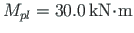
The two load cases depicted in
Fig. 8.11 are applied:
 needed for a moment
 to appear at node 1.
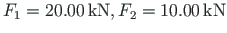
We find that a plastic moment will form at node 1 if the load factor
to appear at node 1.
We find that a plastic moment will form at node 1 if the load factor
 as shown in Fig. 8.5(a)
(
as shown in Fig. 8.5(a)
(
 (deltaM0)
was found on page
(deltaM0)
was found on page 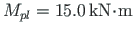 are added to the ends of elements 3 and 4 at plastic hinges 4 and 5.
Similarly attached to the ends of elements 2 and 3 at plastic hinge 3, are
the boundary moments that are equal to the full plastic moment
are added to the ends of elements 3 and 4 at plastic hinges 4 and 5.
Similarly attached to the ends of elements 2 and 3 at plastic hinge 3, are
the boundary moments that are equal to the full plastic moment
 (see excerpt 8.12).
The corresponding load factor
(see excerpt 8.12).
The corresponding load factor
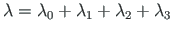 is shown in Fig. 8.5(b).
We now find that at node 1, a fourth full plastic moment
is shown in Fig. 8.5(b).
We now find that at node 1, a fourth full plastic moment
 forms (see Fig. 8.5(b)).
Making use of the EST method described in Chapter 3, ``Statically indeterminate problems'', we carry out the following steps of calculations:
1. Input data for the GNU Octave program spESTframeSn0LaheWFI.m are given in excerpts from the program: element and nodal loads - excerpt 8.10; nodal coordinates - excerpt 8.11; element properties, topology and hinges - excerpt 8.12.
 Number_of_frame_nodes=5
 Number_of_elements=4
 Number_of_support_reactions=5
 spNNK=12*Number_of_elements+Number_of_support_reactions;
 Number_of_unknowns=spNNK
 Displacements and forces are calculated on parts ''Nmitmeks'' of the element
 Nmitmeks=4
 Lp=10.0; % graphic axis
# ---- Load variants -----
load_variant=1;
#load_variant=2;
# --- Element properties ---
 EIp=20000 # kN/m^2
 EIr=40000 # kN/m^2
 EAp=4.6*10^6
#EAp=4.6*10^15;
 EAr=6.8*10^6
#EAr=6.8*10^15;
 GAp=0.4*EAp
 GAr=0.4*EAr
 baasi0=EIp/4  # scaling multiplier for displacements
# baasi0=1.0;
h=4.0;
l=4.0;
l1=l   % l
l2=l   % l
Mplr=30.0 # The plastic moment of beam
Mplp=15.0 # The plastic moment of column
# Loads
F2s=0.5;
F3s=1.0;
switch (koormusvariant)

case{1}
disp('---  ')
disp(' Load variant 1 ')
disp('---  ')
#
disp('deltaM0=15.0-AbsmaxminM ')
disp(' myfile11.mat Flambda Flambda0 Flambda1 Flambda2 deltaM0 muutujaDaF3  ')
disp('load  myfile11.mat ')
load myfile11.mat
#
Flambda
Flambda0
Flambda1
Flambda2
deltaM0
muutujaDaF3
#
# Element load  in local coordinates
#  qz     qx     qA      qL
# Uniformly distributed load in local coordinate z and x directions
Loadsq on element=4;
esQkoormus=zeros(LoadsqONelement,4,ElementideArv);
esQkoormus(1,1:4,1)=[0.0 0.0 0.0 4.0];
esQkoormus(1,1:4,2)=[0.0 0.0 0.0 4.0];
esQkoormus(1,1:4,3)=[0.0 0.0 0.0 4.0];
esQkoormus(1,1:4,4)=[0.0 0.0 0.0 4.0];
#
# Point load in local coordinate z and x directions  kN
#  Fz, Fx, aF (coordinate of the point of force application)
LoadsF on Element=5;
esFjoud=zeros(LoadsF_on_Element,2,ElementideArv);
esFjoud(1,1:3,1)=[0.0 0.0 4.0];
esFjoud(1,1:3,2)=[0.0 0.0 4.0];
#esFjoud(2,1:3,2)=[0.0 0.0 4.0];
esFjoud(1,1:3,3)=[0.0 0.0 4.0];
esFjoud(1,1:3,4)=[0.0 0.0 4.0];
#
# Node forces in global coordinates
# sSolmF(forces,1,nodes); forces=[Fx; Fz; My]
sSolmF = zeros(3,1,SolmedeArv);
#sSolmF(:,1,1)= 0.0;
sSolmF(1,1,2)= F2s; # 0.5;
sSolmF(2,1,3)= F3s; # 1.0;
#sSolmF(:,1,4)= 0.0
#sSolmF(:,1,5)= 0.0
#
#s1F(1,1,1)=0.0;  # force Fz
#s1F(2,1,1)=0.0;  # force Fz
#s1F(3,1,1)=0.0;  # force My


# Support shift - tSiire#
# Support shift is multiplied by scaling multiplier
tSiire = zeros(3,1,SolmedeArv);
#tSiire(:,1,1)= 0.0
#tSiire(2,1,1)= 0.01*baasi0
#tSiire(:,1,2)= 0.0
#tSiire(:,1,3)= 0.0
#tSiire(:,1,4)= 0.0
#tSiire(:,1,5)= 0.0
case{2}
disp('---  ')
disp(' Load variant 2 ')
disp('---  ')
disp(' load myfile00.mat  ')
load myfile00.mat
disp(' plastF1F2;  ')
#disp('plastF1F2=[Flambda Flambda0 Flambda1 Flambda2 Flambda3 F2s00 F3s00] ')
plastF1F2;
Flambda=plastF1F2(1,1)
Flambda0=plastF1F2(1,2)
Flambda1=plastF1F2(1,3)
Flambda2=plastF1F2(1,4)
Flambda3=plastF1F2(1,5)
F2s00=plastF1F2(1,6)
F3s00=plastF1F2(1,7)
#
# Element load  in local coordinates
#  qz     qx     qA      qL
# Uniformly distributed load in local coordinate z and x directions
Loadsq on element=4;
esQkoormus=zeros(LoadsqONelement,4,ElementideArv);
esQkoormus(1,1:4,1)=[0.0 0.0 0.0 4.0];
esQkoormus(1,1:4,2)=[0.0 0.0 0.0 4.0];
esQkoormus(1,1:4,3)=[0.0 0.0 0.0 4.0];
esQkoormus(1,1:4,4)=[0.0 0.0 0.0 4.0];
#
# Point load in local coordinate z and x directions  kN
#  Fz, Fx, aF (coordinate of the point of force application)
LoadsF on Element=5;
esFjoud=zeros(LoadsF_on_Element,2,ElementideArv);
esFjoud(1,1:3,1)=[0.0 0.0 4.0];
esFjoud(1,1:3,2)=[0.0 0.0 4.0];
#esFjoud(2,1:3,2)=[0.0 0.0 4.0];
esFjoud(1,1:3,3)=[0.0 0.0 4.0];
esFjoud(1,1:3,4)=[0.0 0.0 4.0];
#
# Node forces in global coordinates
# sSolmF(forces,1,nodes); forces=[Fx; Fz; My]
sSolmF = zeros(3,1,SolmedeArv);
#sSolmF(:,1,1)= 0.0;
sSolmF(1,1,2)= F2s00;
sSolmF(2,1,3)= F3s00;
#sSolmF(:,1,4)= 0.0
#sSolmF(:,1,5)= 0.0
#
#s1F(1,1,1)=0.0;  # force Fz
#s1F(2,1,1)=0.0;  # force Fz
#s1F(3,1,1)=0.0;  # force My


# Support shift - tSiire#
# Support shift is multiplied by scaling multiplier
tSiire = zeros(3,1,SolmedeArv);
#tSiire(:,1,1)= 0.0
#tSiire(2,1,1)= 0.01*baasi0
#tSiire(:,1,2)= 0.0
#tSiire(:,1,3)= 0.0
#tSiire(:,1,4)= 0.0
#tSiire(:,1,5)= 0.0
otherwise
disp(' No load variant cases ')
endswitch
#==========
#     Nodal coordinates
#==========
krdn=[#  x       z
        0.0     0.0;    % node 1
        0.0    -4.0;    % node 2
        4.0    -4.0;    % node 3
        8.0    -4.0;    % node 4
        8.0     0.0];   % node 5
#==========
#
#==========
#  Restrictions on support displacements (on - 1, off - 0)
# Support  No   u   w  fi
#==========
tsolm=[1       1 1 1;	% node 1
       5       1 1 0];	% node 5
#==========
# ------------- Element properties, topology and hinges ---------
elasts=[# Element properties
#            n2 - end of the element
#                  n1 - beginning of the element
#                       N, Q, M - hinges at the end of the element
#                                N, Q, M - hinges at the beginning of the element
#                                      Mpl - plastic moment at the end of the element
#                                               Mpl - plastic moment at the beginning
#                                                                      of the element
 EIp EAp GAp   2     1    0 0 0    0 0 0   0.0   0.0 ;    % element 1
 EIr EAr GAr   3     2    0 0 0    0 0 1   Mplr  0.0 ;    % element 2
 EIr EAr GAr   4     3    0 0 1    0 0 1  -Mplp -Mplr ;   % element 3
 EIp EAp GAp   5     4    0 0 1    0 0 1   Mplp  Mplp ];  % element 4
# 1 - hinge 'true' (axial, shear, moment hinges)
#
2. Assembling and solving the boundary problem equations (8.4), carried out by the function
LaheFrameSnDFIm(baasi0,Ntoerkts,esQkoormus,esFjoud,sSolmF,tsolm,tSiire, krdn,selem).
This function gives the unscaled initial parameter vectors of the elements and support reactions according to the load cases.
3. Output data.
Load case 1. The load factor
 (Flambda), forces
  (F3s00) and
 (F2s00) are shown in excerpt 8.13 from the computing diary.
muutujaDaF3 = 12
--------------
deltaM0 =  6.6000
--------------
absX =  6
Flambda3=deltaM0/absX
Flambda3 =  1.1000
Flambda=Flambda0+Flambda1+Flambda2+Flambda3
Flambda =  20
--------------
 F2s01=Flambda*F2s
F2s00 =  10
 F3s01=Flambda*F3s
F3s00 =  20
==============
plastF1F2=[Flambda Flambda0 Flambda1 Flambda2 Flambda3 F2s00 F3s00]
plastF1F2 =

   20.0000   14.6853    3.1993    1.0154    1.1000   10.0000   20.0000

save myfile00.mat plastF1F2
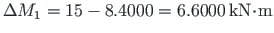
The bending moments in the first loading case are given in excerpt 8.2 from the computing diary, and the bending moments diagram is shown in Fig. 8.3(a).
Moments at nodes (Sign Convention 2)
==============================================================
 Node    Moment DaF No  Fi/baasi0  DaF No   Work_b    Element
--------------------------------------------------------------
   1    6.00000   12   0.00000e+00    9   0.00000e+00    1
   2   -4.00000    6  -1.00000e-03    3   4.00000e-03    1
   2    4.00000   24  -1.00000e-03   21  -4.00000e-03    2
   3    0.00000   18  -1.13333e-03   15  -0.00000e+00    2
   3    0.00000   36   1.08889e-03   33   0.00000e+00    3
   4    0.00000   30   1.08889e-03   27   0.00000e+00    3
   4    0.00000   48  -5.33333e-04   45  -0.00000e+00    4
   5    0.00000   42  -5.33333e-04   39  -0.00000e+00    4
--------------------------------------------------------------
Load case 2. The bending moments in the second loading case are given in excerpt 8.15 from the computing diary, and nowthe bending moments diagram is shown in Fig. 8.5(b).
Moments at nodes (Sign Convention 2)
==============================================================
 Node    Moment DaF No  Fi/baasi0  DaF No   Work_b    Element
--------------------------------------------------------------
   1   15.00000   12   0.00000e+00    9   0.00000e+00    1
   2   -5.00000    6  -2.00000e-03    3   1.00000e-02    1
   2    5.00000   24  -2.00000e-03   21  -1.00000e-02    2
   3   30.00000   18  -1.16667e-03   15  -3.50000e-02    2
   3  -30.00000   36   1.27778e-03   33  -3.83333e-02    3
   4  -15.00000   30   1.77778e-03   27  -2.66667e-02    3
   4   15.00000   48  -6.66667e-04   45  -1.00000e-02    4
   5   15.00000   42  -6.66667e-04   39  -1.00000e-02    4
--------------------------------------------------------------
  At node 4, the dissipation
   D = -(-3.83333e-02 -3.83333e-02) =  0.07667  > 0
  At node 4, the dissipation
   D = -(-2.66667e-02 -1.00000e-02) =  0.03667  > 0
  At node 5, the dissipation
   D = -(-1.00000e-02) =  0.01000 > 0
 ,
,
 ,
,
 .
.
We have found the collapse load factor
 at which the frame will actually fail (see Fig. 8.5(b)).
![\includegraphics[width=65mm]{joonised/raamPiirk8eSn.eps}](img1420xx.png)
![\includegraphics[width=74mm]{joonised/raamPiirk9eSn.eps}](img1422xx.png)