2.3 Equations of joint equilibrium

With joint equilibrium equations, the same transformation matrices of Eqs. (2.6) and (2.9) are used as by writing the compatibility equations. The sum of the internal reactions acting on either side of the cut surface (section) is equal to zero:

$$\left[\begin{array}{c} N^{\left( i\right) }_{element} \\ Q^{\lef... ...eft( i\right)}_{node} \\ M^{\left( i\right) }_{node} \end{array}\right] \qquad$$ (2.30)

The internal reactions acting on either side of the cut surface are equal and opposite. We use Sign Convention 2 for the frame elements.

The equilibrium equations set the sum of the internal reactions in Fig. 1.12 (contact forces^2.5) equal to the externally applied loads $\mathbf{\mathcal{F}_{ext}}$ at joints or node points. We will call the internal reactions contact forces and contact moments.

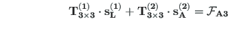
Equilibrium of joint A3 (see Fig. 2.9). The sum of the contact forces $N^{\left( 1\right) }_{L}$, $Q^{\left( 1\right) }_{L}$, $M^{\left( 1\right) }_{L}$ of element 1 and $N^{\left( 2\right) }_{L}$, $Q^{\left( 2\right) }_{L}$, $M^{\left( 2\right) }_{L}$ of element 2 is equal to the external forces $F_{x}$, $F_{z}$, $\mathcal{M}_{y}$ at rigid joint A3, respectively.

Figure 2.9: Equilibrium of joint A3

$$\left[ \begin{array}{ccc} 0 & 1 & 0 \\ - 1 & 0 & 0 \\ 0 & 0 & 1... ...{A} \\ Q^{\left( 2\right)}_{A} \\ M^{\left( 2\right) }_{A} \end{array}\right]$$

$$= \left[\begin{array}{c} F_{x} \\ F_{z} \\ \mathcal{M}_{y} \end{array}\right] \qquad$$ (2.31)

or

$$\hspace*{65pt} \mathbf{T^{\left( 1\right)}_{3\times 3}}\cdot \mat... ...{3\times 3}}\cdot \mathbf{s^{\left( 2\right) }_{A}} = \mathbf{\mathcal{F}_{A3}}$$ (2.32)

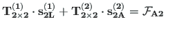
Equilibrium of joint A2 (see Fig. 2.10). The sum of the contact forces $N^{\left( 1\right) }_{L}$, $Q^{\left( 1\right) }_{L}$ of element 1 and $N^{\left( 2\right) }_{L}$, $Q^{\left( 2\right) }_{L}$ of element 2 is equal to the external forces $F_{x}$, $F_{z}$ at hinged joint A3, respectively.

Figure 2.10: Equilibrium of joint A2

$$\left[ \begin{array}{cc} 0 & 1 \\ - 1 & 0 \end{array} \right] \l... ...rray}{c} N^{\left( 2\right)}_{A} \\ Q^{\left( 2\right)}_{A} \end{array}\right]$$

$$= \left[\begin{array}{c} F_{x} \\ F_{z} \end{array}\right] \quad$$ (2.33)

or

$$\mathbf{T^{\left( 1\right)}_{2\times 2}}\cdot \mathbf{s^{\left( 1... ...t \mathbf{s^{\left( 2\right) }_{2A}} = \mathbf{\mathcal{F}_{A2}} \hspace*{20pt}$$ (2.34)

        

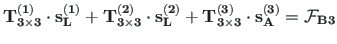
Equilibrium of joint B3 (see Fig. 2.11). The sum of the contact forces $N^{\left( 1\right) }_{L}$, $Q^{\left( 1\right) }_{L}$, $M^{\left( 1\right) }_{L}$ of element 1, $N^{\left( 2\right) }_{L}$, $Q^{\left( 2\right) }_{L}$, $M^{\left( 2\right) }_{L}$ of element 2, and $N^{\left( 3\right) }_{A}$, $Q^{\left( 1\right) }_{A}$, $M^{\left( 3\right) }_{A}$ of element 3 is equal to the external forces $F_{x}$, $F_{z}$, $\mathcal{M}_{y}$ at rigid joint B3, respectively.

Figure 2.11: Equilibrium of joint B3

$$%\hspace*{-135pt} \left[ \begin{array}{ccc} 1 & 0 & 0 \\ 0 & 1 &... ...L} \\ Q^{\left( 1\right) }_{L} \\ M^{\left( 1\right) }_{L} \end{array}\right] \left[ \begin{array}{ccc} 0 & 1 & 0 \\ -1 & 0 & 0 \\ 0 & 0 & 1 ... ...L} \\ Q^{\left( 2\right) }_{L} \\ M^{\left( 2\right) }_{L} \end{array}\right]$$

$$\hspace*{-35pt} + %& + & \left[ \begin{array}{ccc} 1 & 0 & 0 \\ ... ...A} \\ Q^{\left( 3\right) }_{A} \\ M^{\left( 3\right) }_{A} \end{array}\right] = \left[\begin{array}{c} F_{x} \\ F_{z} \\ \mathcal{M}_{y} \end{array}\right]~\qquad\qquad$$ (2.35)

or

$$\mathbf{T^{\left( 1\right)}_{3\times 3}}\cdot \mathbf{s^{\left( 1... ...{3\times 3}}\cdot \mathbf{s^{\left( 3\right) }_{A}} = \mathbf{\mathcal{F}_{B3}}$$ (2.36)

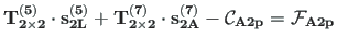
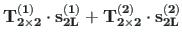
Equilibrium of joint B2 (see Fig. 2.12). The sum of the contact forces $N^{\left( 1\right) }_{L}$, $Q^{\left( 1\right) }_{L}$ of element 1, $N^{\left( 2\right) }_{L}$, $Q^{\left( 2\right) }_{L}$ of element 2, and $N^{\left( 3\right) }_{A}$, $Q^{\left( 1\right) }_{A}$ of element 3 is equal to the external forces $F_{x}$, $F_{z}$ at hinged joint B2, respectively.

Figure 2.12: Equilibrium of joint B2

$$\left[ \begin{array}{cc} 1 & 0 \\ 0 & 1 \end{array} \right] \lef... ...ay}{c} N^{\left( 2\right) }_{L} \\ Q^{\left( 2\right) }_{L} \end{array}\right]$$

$$+ \left[ \begin{array}{ccc} 1 & 0 \\ 0 & 1 \end{array} \right] \... ...rray}\right] = \left[\begin{array}{c} F_{x} \\ F_{z} \end{array}\right] \qquad$$ (2.37)

or

$$\mathbf{T^{\left( 1\right)}_{2\times 2}}\cdot \mathbf{s^{\left( 1... ...mathbf{T^{\left( 2\right)}_{2\times 2}}\cdot \mathbf{s^{\left( 2\right) }_{2L}}$$

$$+ \mathbf{T^{\left( 3\right)}_{2\times 2}}\cdot \mathbf{s^{\left( 3\right) }_{2A}} = \mathbf{\mathcal{F}_{B2}}$$ (2.38)

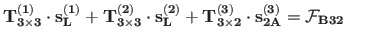
Equilibrium of joint B32 (see Fig. 2.13). The sum of the contact forces $N^{\left( 1\right) }_{L}$, $Q^{\left( 1\right) }_{L}$, $M^{\left( 1\right) }_{L}$ of element 1, $N^{\left( 2\right) }_{L}$, $Q^{\left( 2\right) }_{L}$, $M^{\left( 2\right) }_{L}$ of element 2, and $N^{\left( 3\right) }_{A}$, $Q^{\left( 1\right) }_{A}$ of element 3 is equal to the external forces $F_{x}$, $F_{z}$, $\mathcal{M}_{y}$ at rigid-hinged joint B3, respectively.

$$\left[ \begin{array}{ccc} 1 & 0 & 0 \\ 0 & 1 & 0 \\ 0 & 0 & 1 \... ...t[\begin{array}{c} F_{x} \\ F_{z} \\ \mathcal{M}_{y} \end{array}\right] \quad$$ (2.39)

or

$$\mathbf{T^{\left( 1\right)}_{3\times 3}}\cdot \mathbf{s^{\left( 1... ...2}}\cdot \mathbf{s^{\left( 3\right) }_{2A}} = \mathbf{\mathcal{F}_{B32}} \qquad$$ (2.40)

Figure 2.13: Equilibrium of joint B32

In Fig. 2.13, the three elements are gathered together at the joint with a rigid and pin connection. Unlike compatibility equations, the number of equilibrium equations at the joint does not depend on the number of elements at the joint (see p. ).

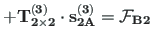
Equilibrium of joint A3s (see Fig. 2.14). The external reactions $C_{x}$, $C_{z}$, $C_{y}$ at the support node are described in global coordinates. The direction of external reactions at the joint is opposite to the direction of internal reactions at the joint and equal to the direction of the external forces $F_{x}$, $F_{z}$, $\mathcal{M}_{y}$ (not shown in Fig. 2.14) at the joint.

Figure 2.14: Equilibrium of support node A3s

$$\left[ \begin{array}{ccc} 0 & 1 & 0 \\ - 1 & 0 & 0 \\ 0 & 0 & 1... ...A} \\ Q^{\left( 1\right) }_{A} \\ M^{\left( 1\right) }_{A} \end{array}\right] \left[ \begin{array}{ccc} \cos\alpha & -\cos\beta & 0 \\ \cos\be... ...{A} \\ Q^{\left( 2\right)}_{A} \\ M^{\left( 2\right) }_{A} \end{array}\right]$$

$$- \left[\begin{array}{c} C_{x} \\ C_{z} \\ C_{y} \end{array}\righ... ...[\begin{array}{c} F_{x} \\ F_{z} \\ \mathcal{M}_{y} \end{array}\right] \qquad$$ (2.41)

or

$$\qquad \mathbf{T^{\left( 1\right)}_{3\times 3}}\cdot \mathbf{s^{\... ... 3}}\cdot \mathbf{\mathcal{C}_{A3s}} = \mathbf{\mathcal{F}_{A3s}} \qquad \qquad$$ (2.42)

Figure 2.15: Equilibrium of support node A2v

$$\left[ \begin{array}{cc} 0 & 1 \\ - 1 & 0 \end{array} \right] \l... ...rray}{c} N^{\left( 6\right)}_{A} \\ Q^{\left( 6\right)}_{A} \end{array}\right]$$

$$- \left[\begin{array}{c} C_{1} \\ C_{2} \end{array}\right] = \left[\begin{array}{c} F_{x} \\ F_{z} \end{array}\right] \quad$$ (2.43)

or

$$\qquad \mathbf{T^{\left( 1\right)}_{2\times 2}}\cdot \mathbf{s^{\... ...eft( 6\right) }_{2A}} - \mathbf{\mathcal{C}_{A2v}} = \mathbf{\mathcal{F}_{A2v}}$$ (2.44)

Figure 2.16: Equilibrium of support node A2p

$$\left[ \begin{array}{cc} 0 & -1 \\ 1 & 0 \end{array} \right] \le... ...rray}{c} N^{\left( 7\right)}_{A} \\ Q^{\left( 7\right)}_{A} \end{array}\right]$$

$$- \left[\begin{array}{c} {\ldots } \\ C_{3} \end{array}\right] = \left[\begin{array}{c} F_{x} \\ F_{z} \end{array}\right] \quad$$ (2.45)

or

$$\mathbf{T^{\left( 5\right) }_{2\times 2}}\cdot \mathbf{s^{\left( ... ...eft( 7\right) }_{2A}} - \mathbf{\mathcal{C}_{A2p}} = \mathbf{\mathcal{F}_{A2p}}$$ (2.46)

The program selects the row index and finds column and element indexes (see excerpts 2.1 and 2.2 from the computing diary). It inserts the joint equilibrium equations into Eq. (2.1). The transformation matrix is inserted with the command cmd = spA=spInsertBtoA(spA,45,22,SpTM3x3); (see excerpt 2.4).

Computing diary excerpt 2.4 ( spESTframe93LaheWFI.m )  

#====================================================================
 Compatibility equations of displacements are inserted into spA  
compatibility_equations_rows =  12
non_zero_elements_in_compatibility_equations =  34 
#====================================================================
 Joint equilibrium equations at nodes 
From_rows = Joint equilibrium equations begin from row: 43
#==================================================================== 
Node =  1
 Number of reactions at the node (node_no, reactions): 1, 2
cmd = spA=spInsertBtoA(spA,43,10,SpTM2x2);
cmd = spA=spInsertBtoA(spA,43,61,SpTM2x2xz);
---------------------------------------------------------
Node =  2
cmd = spA=spInsertBtoA(spA,45,22,SpTM3x3);
cmd = spA=spInsertBtoA(spA,45,4,SpTM3x3);
 Nodal forces at the node
cmd = B(45:47,1)=sSolmF(1:3,2);
---------------------------------------------------------
Node =  3
 Number of reactions at the node (node_no, reactions): 3, 3 
cmd = spA=spInsertBtoA(spA,48,34,SpTM3x3);
cmd = spA=spInsertBtoA(spA,48,63,SpTM3x3xz);
---------------------------------------------------------
Node =  4
cmd = spA=spInsertBtoA(spA,51,46,SpTM3x3);
cmd = spA=spInsertBtoA(spA,51,28,SpTM3x3);
cmd = spA=spInsertBtoA(spA,51,16,SpTM3x3);
 Nodal forces at the node
cmd = B(51:53,1)=sSolmF(1:3,4);
---------------------------------------------------------
Node =  5
 Number of reactions at the node (node_no, reactions): 5, 2
cmd = spA=spInsertBtoA(spA,54,52,SpTM2x2);
cmd = spA=spInsertBtoA(spA,54,66,SpTM2x2xz);
---------------------------------------------------------
Node =  6
cmd = spA=spInsertBtoA(spA,56,58,SpTM3x3);
cmd = spA=spInsertBtoA(spA,56,40,SpTM3x3);
 Nodal forces at the node
cmd = B(56:58,1)=sSolmF(1:3,6);
#====================================================================
spA_rows =  58
spA_cols =  67
spA_nnz = non_zero_elements_in_spA: 172
  
-----Equilibrium equations are inserted into spA  ----  
  
equilibrium_equations_rows =  16
non_zero_elements_in_equilibrium_equations =  43
#====================================================================