1.3 The system equations of a frame

The total number of unknowns $N_{totl}$ in this problem is decomposed as follows:

• $N_{est}$ - the number of displacements and forces (see Eq. (1.50)) of the elements,
  • for frames = $N_{elemts} \times 12$ ($N_{elemts}$ - the number of elements),
  • for beams = $N_{elemts} \times 8$;
• $N_{react}$ - the number of external support reactions of the frame (beam).

$$N_{totl} = N_{est} + N_{react}$$ (1.53)

To solve this boundary value problem, it is necessary but not sufficient that the number of linear equations $N_{eqs}$ in a system of equations

$$\mathbf{spA}{\cdot}\mathbf{Z} = \mathbf{B} <tex2html_comment_mark>$$ (1.54)

be

$$N_{eqs} = N_{totl}, \hspace*{8pt}\mathrm{and} \hspace*{8pt} \mathrm{rank}\left(spA\right) = N_{totl}$$ (1.55)

Both external and internal boundary conditions (Fig. 1.13) of a system (frame/beam) should be well posed.

The kinematic and static boundary conditions of the external support shown in Fig. (1.10) and these of the internal support shown in Fig. (1.12) should be well posed.

The kinematic and static boundary conditions of the internal support are divided into

• compatibility equations of the displacements at nodes,
• joint equilibrium equations at nodes,
• side conditions (bending moment, axial and shear force hinges)

Figure 1.13: Structure of the system of boundary value problem equations

It is convenien to use a sparse representation of equations (1.54) (see section A.1).

Numerical difficulties may occur when the transfer matrix manipulation involves differences of large numbers, which can lead to inaccuracies in computations [PW94], [PL63]. In the state vector $\mathbf{Z}$ of equations (1.47) the displacements and rotations are small in comparison with the contact forces and moments. We will scale (multiply) the displacements and rotations by 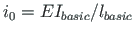$i_{0}= EI_{basic}/l_{basic}$ (as a scaling multiplier for the displacements, basic stiffness is taken).

In the sparse matrix $\mathbf{spA}$ of Eq. (1.54), the basic equations of the system are described in local coordinates. The compatible equations of displacements, joint equilibrium equations, side conditions equations and external support reactions of the system of Eq. (1.54) are described in global coordinates.

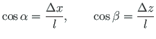
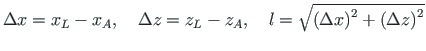
The following direction cosines allow us to transform vectors from local to global coordinates. The direction cosines of a vector are the cosines of the angles between the vector and the coordinate axes (see Fig. 1.14):

$$\cos \alpha = \frac{\Delta x}{l}, \qquad \cos \beta = \frac{\Delta z}{l}$$ (1.56)

Here,

$$\Delta x = x_{L} - x_{A}, \quad \Delta z = z_{L} - z_{A}, \quad l = \sqrt{\left(\Delta x\right)^{2} + \left(\Delta z\right)^{2}}$$ (1.57)

and $x_{A}$, $z_{A}$, $x_{L}$, $z_{L}$ are the start point and the end point coordinates (Fig. 1.14).

Figure 1.14: Angles between the vector and the coordinate axes

The two-dimensional transformation matrix $\mathbf{T_{2\times 2}}$ (considered in section A.2) transforms the vector from local to global coordinates.

$$\mathbf{T_{2\times 2}} = \left[\begin{array}{cc} \cos\alpha & - \cos\beta \\ \cos\beta & \cos\alpha \end{array} \right]$$ (1.58)

The three-dimensional transformation matrix $\mathbf{T_{3\times 3}}$ (considered in section A.2) transforms the vector from local to global coordinates.

$$\mathbf{T_{3\times 3}} = \left[\begin{array}{ccc} \cos\alpha & - \cos\beta & 0 \\ \cos\beta & \cos\alpha & 0 \\ 0 & 0 & 1 \end{array} \right]$$ (1.59)

Note that it is possible to insert the transformation matrices of Eqs. (A.25) and (1.59) into the sparse matrix of Eq. (1.54) with the function spA=spInsert BtoA(spA,M,N,spTi) (p. ).