6.2 Illustrative frame problem 1

Example 6.1 Problem Statement. Figure 6.1 shows a frame of the span length $l = 6{\,}\mathrm{m}$ , carrying a uniform load $q = 20{\,}\mathrm{kN/m}$ . The $5{\,}\mathrm{m}$ long column 3-4 and the $2.5{\,}\mathrm{m}$ long column 2-3 are both loaded with a vertical force $F = 800{\,}\mathrm{kN}$ . At node 2, a horizontal force $H = 90{\,}\mathrm{kN}$ acts.

**Figure 6.1:** The frame EST1
$\includegraphics[width=90mm]{joonised/raamn1moe.eps}$

We assume that the value of the column flexural rigidity $EI_{p} = 2\cdot10^{4} {\,}\mathrm{kN}\hspace*{-2pt}\cdot\hspace*{-2pt}\mathrm{m}^{2}$ and that of the beam $EI_{r} = 1.5EI_{p}$ ( $I_{1} = 1.5{\,}I_{2}$ ); axial rigidity of the columns $EAp=2.0\cdot10^{20}{\,}\mathrm{kN}$ and that of the beam $EAr=2.0\cdot10^{20}{\,}\mathrm{kN}$ ; shear rigidity of the columns $GAp=1.0\cdot10^{25}$ and that of the beam $GAr=1.0\cdot10^{25}$ .

We wish to compute the displacements, reactions, internal forces, and draw the axial force, shear force and bending moment diagrams.

Problem Solving. To solve the problem, we use the EST method. The solving procedure includes the following.

Data input: the number of frame nodes, elements, support reactions; element properties, element loads in local coordinates, node forces in global coordinates, nodal coordinates, topology and hinges, restrictions on support displacements.

$\displaystyle \mathbf{spA}{\cdot}\mathbf{Z} = \mathbf{B}$ (6.5)
Assembling and solving the boundary problem equations (6.1) and (6.5) (prepared and solved by the program). To implement this aim, the program
1. inserts the basic equations of a frame into the equation system,
2. adds the compatibility equations of the displacements at nodes to the equation system,
3. adds the joint equilibrium equations,
4. adds the side conditions (hinges),
5. adds the restrictions on support displacements,
6. solves the system of sparse equations,
7. produces an output: initial parameter vectors for element displacements and forces; support reactions.
Output: element displacements and forces determined by the transfer matrix.

**Figure 6.2:** Numeration of displacements and forces of the frame EST1
$\includegraphics[width=100mm]{joonised/raamny1moe.eps}$

1. Input data for the GNU Octave program yspESTframe1LaheWFI.m are given in excerpts from the program: element and nodal loads - excerpt 6.2; nodal coordinates - excerpt 6.3; element properties, topology and hinges - excerpt 6.4.

Program excerpt 6.2 ( ''Nmitmeks'' yspESTframe1LaheWFI.m )

 epsdountil=0.0000001; # for iteration (max |S| increment)
 Number_of_frame_nodes=4 
 Number_of_elements=3
 Number_of_support_reactions=5
 spNNK=12*Number_of_elements+Number_of_support_reactions;
 Number_of_unknowns=spNNK 
 Displacements and forces are calculated on parts ''Nmitmeks'' of the element
 Nmitmeks=4 
# --- Element properties ---

  
 EIp=20000; # kN/m^2
 EIr=40000; # kN/m^2
# EAp=4.6*10^6; 
 EAp=2.0^20; 
# EAp=4.6*10^6; 
 EAr=6.8*10^20;
# EAr=6.8*10^6;
 GAp=1.0e+25;
 GAr=1.0e+25;
# GAp=0.4*EAp; 
# GAr=0.4*EAr;

baasi0=EIp/5 # scaling multiplier for displacements # baasi0=1.0; # Element load in local coordinates # qz qx qA qL # Uniformly distributed load in local coordinate z and x directions LoadsqONelement=4; esQkoormus=zeros(LoadsqONelement,4,ElementideArv);

baasi0=EIp/5  # scaling multiplier for the displacements
esQkoormus(1,1:4,1)=[0.0 0.0 0.0 5.0]; 
esQkoormus(1,1:4,2)=[20.0 0.0 0.0 6.0];
esQkoormus(1,1:4,3)=[0.0 0.0 0.0 2.5];

# # Point load in local coordinate z and x directions kN # Fz, Fx, aF (coordinate of the point of force application) LoadsF_on_Element=5; esFjoud=zeros(LoadsF_on_Element,2,ElementideArv);

esFjoud(1,1:3,1)=[0.0 0.0 5.0];
esFjoud(1,1:3,2)=[0.0 0.0 6.0];  
esFjoud(1,1:3,3)=[0.0 0.0 2.5];

# # Node forces in global coordinates # sSolmF(forces,1,nodes); forces=[Fx; Fz; My] sSolmF = zeros(3,1,SolmedeArv);

#sSolmF(:,1,1)= 0.0
sSolmF(2,1,1)= 800.0;  %  Fz
sSolmF(1,1,2)= -90.0;  %  Fx
sSolmF(2,1,2)= 800.0;  %  Fz
#sSolmF(:,1,3)= 0.0
#sSolmF(:,1,4)= 0.0

# #s1F(1,1,1)=0.0; # force Fz #s1F(2,1,1)=0.0; # force Fz #s1F(3,1,1)=0.0; # force My # Support shift - tSiire# # Support shift is multiplied by scaling multiplier tSiire = zeros(3,1,SolmedeArv);

#tSiire(:,1,1)= 0.0
#tSiire(2,1,1)= 0.01*baasi0
#tSiire(:,1,2)= 0.0
#tSiire(:,1,3)= 0.0
#tSiire(:,1,4)= 0.0

Program excerpt 6.3 ( yspESTframe1LaheWFI.m )
#========== # Nodal coordinates #========== krdn=[# x z 0.0 0.0; % node 1 6.0 0.0; % node 2 6.0 2.5; % node 3 0.0 5.0]; % node 4 #========== #========== # Restrictions on support displacements (on - 1, off - 0) # Support No u w fi #========== tsolm=[3 1 1 0; % node 3 4 1 1 1]; % node 4 #==========

Program excerpt 6.4 ( yspESTframe1LaheWFI.m )
# ------------- Element properties, topology and hinges --------- elasts=[# Element properties # n2 - end of the element # n1 - beginning of the element # N, Q, M - hinges at the end of the element # N, Q, M - hinges at the beginning of the element # EIp EAp GAp 1 4 0 0 0 0 0 0; % element 1 EIr EAr GAr 2 1 0 0 0 0 0 0; % element 2 EIp EAp GAp 3 2 0 0 1 0 0 0]; % element 3 # 1 - hinge 'true' (axial, shear, moment hinges) #

2. Assembling and solving the boundary problem equations (6.5), carried out by the function Lahe2FrameDFIm(baasi0,Ntoerkts,esQkoormus,esFjoud,sSolmF,tsolm,tSiire, krdn,selem). The program has numbered the displacements and forces of the element ends of the frame as shown in Fig. 6.2.
The results of iteration of the axial forces are shown in excerpt 6.3 from the computing diary.

Computing diary excerpt 6.3 ( yspESTframe1LaheWFI.m )
SIvec = Element Linear 1 2 3 4 5 1 -897.500 -904.385 -904.364 -904.364 -904.364 -904.364 2 -54.000 -55.431 -55.362 -55.362 -55.362 -55.362 3 -822.500 -815.615 -815.636 -815.636 -815.636 -815.636

The unscaled initial parameter vectors of the elements are shown in excerpt 6.4 from the computing diary.

Computing diary excerpt 6.4 ( yspESTframe1LaheWFI.m )
-------- Scaling multiplier for displacements = 1/baasi0 -------- ============================================================================ Unscaled initial parameter vector Element No u w fi S H M ---------------------------------------------------------------------------- 1 -0.000e+00 0.000e+00 0.000e+00 904.364 55.362 -154.733 2 -3.344e-02 2.261e-17 3.342e-04 55.362 -104.364 152.316 3 1.020e-17 3.344e-02 8.548e-03 815.636 34.638 -113.870 ----------------------------------------------------------------------------

The support reactions of the frame in global coordinates are shown in excerpt 6.5 from the computing diary.

Computing diary excerpt 6.5 ( yspESTframe1LaheWFI.m )
Support reactions begin from X row: 37 =========================================== No X Node Cx <=> 1 Cz <=> 2 Cy <=> 3 ------------------------------------------- 37 +3.463836e+01 3 1 38 -8.156356e+02 3 2 39 +5.536164e+01 4 1 40 -9.043644e+02 4 2 41 -1.547333e+02 4 3 --------------------------------------------

         3. Output: the element displacements and forces determined by the transfer matrix are given in excerpt 6.6 from the computing diary.
The bending moment, shear force Q and axial force N diagrams of the frame EST1 are shown in Fig. 6.3.

Figure 6.3: Internal forces diagrams of the frame EST1

$\includegraphics[width=75mm]{joonised/raamnp4iIIe.eps}$
[Axial force N diagram]

$\includegraphics[width=90mm]{joonised/raamnp3iIIe.eps}$
                  [Shear force Q diagram]

$\includegraphics[width=68mm]{joonised/raamnp2iIIe.eps}$
[Bending moment diagram]

                             (bracketed are values of linear solution)

Computing diary excerpt 6.6 ( yspESTframe1LaheWFI.m )
#================================================================================= Element displacements and forces determined by transfer matrix #================================================================================= Displacements and forces of element no 1 of length 5.000 m The element is divided into 4 parts displacement u - 0.00000e+00 -5.65228e-18 -1.13046e-17 -1.69568e-17 -2.26091e-17 displacement w - 0.00000e+00 -5.11088e-03 -1.65057e-02 -2.80093e-02 -3.34392e-02 rotation fi - 0.00000e+00 7.40749e-03 9.99497e-03 7.58070e-03 3.34242e-04 normal force N - -904.36438 -904.36438 -904.36438 -904.36438 -904.36438 shear force Q - -55.36164 -62.06071 -64.40074 -62.21735 -55.66392 moment force M - 154.73331 80.90916 1.40208 -78.20348 -152.31615 ------------------ axial force S - -904.36438 -904.36438 -904.36438 -904.36438 -904.36438 transv force H - -55.36164 -55.36164 -55.36164 -55.36164 -55.36164 ---------------------------------------------------------------------------- Displacements and forces of element no 2 of length 6.000 m The element is divided into 4 parts displacement u - -3.34392e-02 -3.34392e-02 -3.34392e-02 -3.34392e-02 -3.34392e-02 displacement w - 2.26091e-17 3.39304e-03 8.42296e-03 8.39268e-03 3.29397e-10 rotation fi - 3.34242e-04 -3.73960e-03 -2.22252e-03 2.62995e-03 8.54847e-03 normal force N - -55.36164 -55.36164 -55.36164 -55.36164 -55.36164 shear force Q - 104.34587 74.57141 44.48742 14.21878 -16.10888 moment force M - -152.31615 -18.08174 71.24329 115.28819 113.87012 ------------------ axial force S - -55.36164 -55.36164 -55.36164 -55.36164 -55.36164 transv force H - 104.36438 74.36438 44.36438 14.36438 -15.63562 ---------------------------------------------------------------------------- Displacements and forces of element no 3 of length 2.500 m The element is divided into 4 parts displacement u - 1.01954e-17 7.64658e-18 5.09772e-18 2.54886e-18 1.54074e-33 displacement w - 3.34392e-02 2.70705e-02 1.90043e-02 9.79115e-03 7.61059e-11 rotation fi - 8.54847e-03 1.16917e-02 1.39732e-02 1.53568e-02 1.58205e-02 normal force N - -815.63562 -815.63562 -815.63562 -815.63562 -815.63562 shear force Q - -41.61080 -44.17449 -46.03540 -47.16392 -47.54210 moment force M - 113.87012 87.02657 58.79850 29.63498 -0.00000 ------------------ axial force S - -815.63562 -815.63562 -815.63562 -815.63562 -815.63562 transv force H - -34.63836 -34.63836 -34.63836 -34.63836 -34.63836 ----------------------------------------------------------------------------

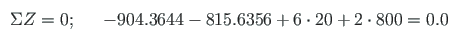
Figure 6.4: Boundary forces of the frame EST1

$\includegraphics[width=90mm]{joonised/raamn1Summoe.eps}$

Testing a static equilibrium for the frame
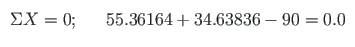
Consider next a static equilibrium of the frame shown in Fig. 6.4. Let us project the forces onto the X-axis,

$\displaystyle \begin{array}{ccl} \Sigma X = 0; & & 55.36164 + 34.63836 - 90 = 0.0 % {{\;}=\hspace*{-1pt}?{\;}} 0 \vspace*{2mm} \\ \end{array}$ (6.6)

and onto the Z-axis,

$\displaystyle \begin{array}{ccl} \Sigma Z = 0; & & - 904.3644 - 815.6356 + 6\cdot20 + 2\cdot 800 = 0.0 \end{array}$ (6.7)

We now write the equation of the sum of the moments and the moments of the forces acting about point 3 shown in Fig. 6.4:

$\displaystyle \Sigma M_{3} = 0;\qquad -154.7333 - 904.3644\cdot 6.0 + 55.36164\cdot 2.5 + 800\cdot 0.0334392 \qquad \qquad$

$\displaystyle + 800\cdot (6.0 + 0.0334392) + 20\cdot 6.0\cdot (3 + 0.0334392)+ ... ...6\cdot 10^{-4}{\,}\mathrm{kN}\hspace*{-2pt}\cdot\hspace*{-2pt}\mathrm{m} \qquad$ (6.8)

The calculations with equations (6.6), (6.7), and (6.8) have verified the static equilibrium of the frame.

Figure 6.5: Elements of the frame EST1

$\includegraphics[width=0.70\textwidth]{joonised/yspESTframe1e.eps}$

Figure 6.6: Sparsity pattern of matrix spA of the frame EST1

$\includegraphics[width=0.72\textwidth]{joonised/yspESTframe1_spars.eps}$

$\includegraphics[width=75mm]{joonised/raamnp4iIIe.eps}$ [Axial force N diagram]
$\includegraphics[width=90mm]{joonised/raamnp3iIIe.eps}$ [Shear force Q diagram]		$\includegraphics[width=68mm]{joonised/raamnp2iIIe.eps}$ [Bending moment diagram]
(bracketed are values of linear solution)

$\displaystyle \Sigma M_{3} = 0;\qquad -154.7333 - 904.3644\cdot 6.0 + 55.36164\cdot 2.5 + 800\cdot 0.0334392 \qquad \qquad$
$\displaystyle + 800\cdot (6.0 + 0.0334392) + 20\cdot 6.0\cdot (3 + 0.0334392)+ ... ...6\cdot 10^{-4}{\,}\mathrm{kN}\hspace{-2pt}\cdot\hspace{-2pt}\mathrm{m} \qquad$			(6.8)