3.2 Illustrative frame problem 2

Example 3.2   Problem Statement. Depicted in Fig. 3.9 is a two-span frame. The height of the frame $h = 7{\,}\mathrm{m}$, the two spans are of the same length: $l = 9{\,}\mathrm{m}$. The rafter 2-4 is loaded with a vertical concentrated load $F = 16{\,}\mathrm{kN}$. The column 3-4 (of length $h_{2} = 5.6{\,}\mathrm{m}$) is loaded with a uniform load $q = 16{\,}\mathrm{kN/m}$.

Figure 3.9: Two-span frame EST93

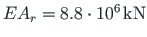
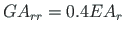
Assume that the value of the column flexural rigidity is $EI_{p} = 2\cdot10^{4} {\,}\mathrm{kN}\hspace*{-2pt}\cdot\hspace*{-2pt}\mathrm{m}^{2}$ and that of the rafter is $EI_{r} = 2.0EI_{p}$ ( $I_{1} = 2.0\cdot I_{2}$); the axial rigidity of the column $EA_{p} = 4.6\cdot 10^{6}{\,}\mathrm{kN}$ and that of the rafter $EA_{r} = 8.8\cdot 10^{6}{\,}\mathrm{kN}$; the shear rigidity of the column 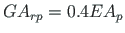$GA_{rp} = 0.4EA_{p}$ and that of the rafter $GA_{rr} = 0.4EA_{r}$.

We wish to compute the displacements, reactions, internal forces, and draw the axial force, shear force and bending moment diagrams.

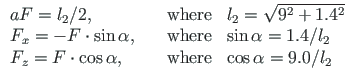
Problem Solving. To solve the problem, the EST method is used. Since the element loads are described in local coordinates, we assume the directions of the local coordinates shown in Fig. 3.10. Now we express the vertical concentrated load $F = 16{\,}\mathrm{kN}$ (see Fig. 3.9 b) in local coordinates ($F_{x}$ - projection onto the x-axis and $F_{z}$ - projection onto the z-axis):

$$\begin{array}{lll} aF = l_{2}/2, &\quad \mathrm{where} & l_{2} = ... ...= F\cdot \cos\alpha, &\quad \mathrm{where} & \cos\alpha = 9.0/l_{2} \end{array}$$ (3.5)

Here, $l_{2}$ is the length of the rafter and $aF = l_{2}/2$ is the force $F$ application point in local coordinates.

Figure 3.10: Numeration of displacements and forces of the two-span frame EST93

As in example 3.1, we carry out the following steps of calculations.

1. Data input: the number of frame nodes, elements, support reactions; element properties, element loads in local coordinates, node forces in global coordinates, nodal coordinates, topology and hinges, restrictions on support displacements.
   
   

   $$\mathbf{spA}{\cdot}\mathbf{Z} = \mathbf{B}$$ (3.6)

   
   
2. Assembling and solving the boundary problem equations (2.1) and (3.6) (prepared and solved by the program). To implement this aim, the program
   1. inserts the basic equations of a frame into the equation system,
   2. adds the compatibility equations of the displacements at nodes to the equation system,
   3. adds the joint equilibrium equations,
   4. adds the side conditions (hinges),
   5. adds the restrictions on support displacements,
   6. solves the compiled system of sparse equations,
   7. produces an output: initial parameter vectors for element displacements and forces; support reactions.
3. Output: element displacements and forces determined by the transfer matrix.

1. Input data for the GNU Octave program spESTframe93LaheWFI.m are shown in excerpts from the program: element and nodal loads - excerpt 3.4; nodal coordinates - excerpt 3.5; element properties, topology and hinges - excerpt 3.6.

Program excerpt 3.4 ( spESTframe93LaheWFI.m )  

 Number_of_frame_nodes=6 
 Number_of_elements=5
 Number_of_support_reactions=7
 spNNK=12*Number_of_elements+Number_of_support_reactions;
 Number_of_unknowns=spNNK 
 Displacements and forces calculated on parts of the element 'Nmitmeks'.
 Nmitmeks=4
 Lp=18.0; # graphics axis 
# --- Element properties ---

  
EIp=20000 # kN/m^2 
EIr=40000 # kN/m^2
# EAp=4.6*10^6 
EAp=4.6*10^15; 
#EAr=6.8*10^6;
EAr=6.8*10^15 
GAp=0.4*EAp;    
GAr=0.4*EAr; 
F2=16;
qz5=16;
L2x=sqrt(9^2+1.4^2); # length of the element
sinA2=1.4/L2x;
cosA2=9.0/L2x;
aF2=L2x/2;
Fz2=F2*cosA2;
Fx2=-F2*sinA2;

 
baasi0=EIp/5.6  # scaling multiplier for displacements
#baasi0=1.0;

#Element load  in local coordinates 
#  qz     qx     qA      qL 
# Uniformly distributed load in local coordinate z and x directions
LoadsqONelement=4;
esQkoormus=zeros(LoadsqONelement,4,ElementideArv);

esQkoormus(1,1:4,1)=[0.0 0.0 0.0 5.6];  
esQkoormus(1,1:4,2)=[0.0 0.0 0.0 L2x];  
esQkoormus(1,1:4,3)=[0.0 0.0 0.0 7.0];  
esQkoormus(1,1:4,4)=[0.0 0.0 0.0 L2x];  
esQkoormus(1,1:4,5)=[qz5 0.0 0.0 5.6];

 
#
# Point load in local coordinate z and x directions  kN
#  Fz, Fx, aF (coordinate of the point of force application)
LoadsF_on_Element=5; 
esFjoud=zeros(LoadsF_on_Element,2,ElementideArv);

esFjoud(1,1:3,1)=[0.0 0.0 5.6];
esFjoud(1,1:3,2)=[Fz2 Fx2 aF2]; 
esFjoud(1,1:3,3)=[0.0 0.0 7.0];  
esFjoud(1,1:3,4)=[0.0 0.0 L2x];
esFjoud(1,1:3,5)=[0.0 0.0 5.6];

 
#
#Node forces in global coordinates
# sSolmF(forces,1,nodes); forces=[Fx; Fz; My]
sSolmF = zeros(3,1,SolmedeArv);

#sSolmF(:,1,1)= 0.0
#sSolmF(:,1,2)= 0.0the
#sSolmF(:,1,3)= 0.0
#sSolmF(:,1,4)= 0.0
#sSolmF(:,1,5)= 0.0
#sSolmF(:,1,6)= 0.0

 
#
#s1F(1,1,1)=0.0;  # force Fz
#s1F(2,1,1)=0.0;  # force Fz
#s1F(3,1,1)=0.0;  # force My


# Support shift - tSiire
# Support shift is multiplied by scaling multiplier
tSiire = zeros(3,1,SolmedeArv);

#tSiire(1,1,1)= 0.0
#tSiire(2,1,1)= 0.01*baasi0  
#tSiire(1,1,3)= 0.0
#tSiire(2,1,3)= 0.0
#tSiire(3,1,3)= 0.0
#tSiire(1,1,5)= 0.0
#tSiire(2,1,5)= 0.0

Program excerpt 3.5 ( spESTframe93LaheWFI.m )  

#==========
#     Nodal coordinates
#==========
krdn=[#  x       z
        0.0     0.0;    # node 1
        0.0    -5.6;    # node 2
        9.0     0.0;    # node 3
        9.0    -7.0;    # node 4
       18.0     0.0;    # node 5
       18.0    -5.6];   # node 6
#========== 
#
#==========
#  Restrictions on support displacements (on - 1, off - 0)
# Support  No   u   w  fi  
#==========       
tsolm=[1     1 1 0;   % node 1
       3     1 1 1;   % node 3
       5     1 1 0];  % node 5       
#==========

Program excerpt 3.6 ( spESTframe93LaheWFI.m )  

# ------------- Element properties, topology and hinges ---------
elasts=[# Element properties 
#            n2 - end of the element 
#                  n1 - beginning of the element
#                       N, Q, M -  hinges at the end of the element
#                                N, Q, M -  hinges at the beginning of the element 
# 
 EIp EAp GAp   2     1    0 0 0    0 0 1;    % element 1
 EIr EAr GAr   4     2    0 0 0    0 0 0;    % element 2
 EIp EAp GAp   4     3    0 0 0    0 0 0;    % element 3
 EIr EAr GAr   6     4    0 0 0    0 0 0;    % element 4
 EIp EAp GAp   5     6    0 0 1    0 0 0];   % element 5
# 1 - hinge 'true' (axial, shear, moment hinges)
#

2. Assembling and solving the boundary problem equations (3.6), carried out by the function LaheFrameDFIm(baasi0,Ntoerkts,esQkoormus,esFjoud, sSolmF,tsolm,tSiire, krdn,selem). The program has numbered the displacements and forces of the frame element ends as shown in Fig. 3.10. The unscaled initial parameter vectors of the elements are shown in excerpt 3.4 from the computing diary.

Computing diary excerpt 3.4 ( spESTframe93LaheWFI.m )  

-------- Scaling multiplier for displacements = 1/baasi0 --------   
============================================================================
 Unscaled initial parameter vector 
Element    u           w           fi               N          Q          M 
  No
----------------------------------------------------------------------------
   1   -0.000e+00   0.000e+00   1.189e-02       22.670     12.850      0.000
   2   -4.721e-02  -7.343e-03   1.815e-03       16.182    -20.426     71.959
   3   -0.000e+00   0.000e+00   0.000e+00       -4.870     27.275   -102.642
   4   -4.721e-02   7.343e-03   2.513e-03       39.371     -7.946     46.197
   5   -2.192e-15   4.778e-02   2.340e-04       -1.800    -40.125    -26.181
----------------------------------------------------------------------------

The support reactions of the frame in global coordinates are shown in excerpt 3.5 from the computing diary.

Computing diary excerpt 3.5 ( spESTframe93LaheWFI.m )  

Support reactions begin from row X: 61  
===========================================
 No         X        Node    Cx <=> 1 
                             Cz <=> 2
                             Cy <=> 3 
------------------------------------------- 
 61   +1.284975e+01    1         1 
 62   -2.267047e+01    1         2 
 63   +2.727509e+01    3         1 
 64   +4.870101e+00    3         2 
 65   -1.026424e+02    3         3 
 66   +4.947516e+01    5         1 
 67   +1.800369e+00    5         2 
--------------------------------------------

3. Output: the element displacements and forces determined by the transfer matrix are shown in excerpt 3.6 from the computing diary.

The bending moment M, shear force Q and axial force N diagrams of the frame EST93 are shown in Fig. 3.11.

Figure 3.11: Internal forces diagrams of the two-span frame EST93

[Bending moment diagram]
[Shear force Q diagram]		[Axial force N diagram]

Computing diary excerpt 3.6 ( spESTframe93LaheWFI.m )  

#=================================================================================
 Element displacements and forces determined by transfer matrix 
#================================================================================= 
Displacements and forces of element no 1 of length 5.600 m 
The element is divided into 4 parts 
 displacement u -  0.00000e+00 -6.89971e-15 -1.37994e-14 -2.06991e-14 -2.75988e-14
 displacement w -  0.00000e+00 -1.63514e-02 -3.09398e-02 -4.20022e-02 -4.77757e-02
 rotation    fi -  1.18894e-02  1.12598e-02  9.37089e-03  6.22270e-03  1.81524e-03
 normal force N - -22.67047   -22.67047   -22.67047   -22.67047  -22.67047
 shear force  Q - -12.84975   -12.84975   -12.84975   -12.84975  -12.84975
 moment force M -   0.00000   -17.98964   -35.97929   -53.96893  -71.95857

 
----------------------------------------------------------------------------
Displacements and forces of element no 2 of length 9.108 m 
The element is divided into 4 parts 
 displacement u - -4.72079e-02 -4.72079e-02 -4.72079e-02 -4.72079e-02 -4.72079e-02
 displacement w - -7.34346e-03 -7.81788e-03 -4.99369e-03  2.77278e+00  2.22079e+01
 rotation    fi -  1.81524e-03 -9.57252e-04 -1.08203e-03 -3.65812e+00 -1.46316e+01
 normal force N -  -16.18166   -16.18166   -13.72234   -13.72234  -13.72234
 shear force  Q -   20.42597    20.42597     4.61611     4.61611    4.61611
 moment force M -  -71.95857   -25.44743    21.06372    31.57487   42.08602
----------------------------------------------------------------------------
Displacements and forces of element no 3 of length 7.000 m 
The element is divided into 4 parts 
 displacement u - 0.00000e+00  1.85276e-15  3.70551e-15  5.55827e-15  7.41102e-15
 displacement w - 0.00000e+00 -6.64042e-03 -2.16891e-02 -3.78371e-02 -4.77757e-02
 rotation    fi - 0.00000e+00  6.89296e-03  9.60943e-03  8.14940e-03  2.51287e-03
 normal force N -    4.87010     4.87010     4.87010     4.87010    4.87010
 shear force  Q -  -27.27509   -27.27509   -27.27509   -27.27509  -27.27509
 moment force M -  102.64244    54.91103     7.17962   -40.55179  -88.28320
 
----------------------------------------------------------------------------
Displacements and forces of element no 4 of length 9.108 m 
The element is divided into 4 parts 
 displacement u - -4.72079e-02 -4.72079e-02 -4.72079e-02 -4.72079e-02 -4.72079e-02
 displacement w -  7.34346e-03  4.22475e-03  4.74885e-03  6.57025e-03  7.34346e-03
 rotation    fi -  2.51287e-03  3.98052e-04 -6.86705e-04 -7.41404e-04  2.33954e-04
 normal force N -  -39.37128   -39.37128   -39.37128   -39.37128  -39.37128
 shear force  Q -    7.94644     7.94644     7.94644     7.94644    7.94644
 moment force M -  -46.19719   -28.10266   -10.00814     8.08639   26.18091
----------------------------------------------------------------------------
Displacements and forces of element no 5 of length 5.600 m 
The element is divided into 4 parts 
 displacement u - -2.19175e-15 -1.64382e-15 -1.09588e-15 -5.47939e-16  0.00000e+00
 displacement w - 4.77757e-02   5.02581e-01  7.35198e+00  3.70545e+01  1.17045e+02
 rotation    fi - 2.33954e-04  -1.30263e+00 -1.04416e+01 -3.52566e+01 -8.35876e+01
 normal force N -    1.80037     1.80037     1.80037     1.80037    1.80037
 shear force  Q -   40.12484    17.72484    -4.67516   -27.07516  -49.47516
 moment force M -   26.18091    66.67568    75.81046    53.58523   -0.00000
----------------------------------------------------------------------------

Figure 3.12: Boundary forces of the two-span frame EST93

Testing a static equilibrium for the frame

Consider a static equilibrium of the frame shown in Fig. 3.12. Let us project the forces onto the X-axis,

$$\begin{array}{ccl} \Sigma X = 0; & & 12.85 + 27.275 + 49.475 - 16\cdot 5.6 = 0 \end{array}\vspace*{-8pt}$$ (3.7)

and onto the Z-axis,

$$\begin{array}{ccl} \Sigma Z = 0; & & 16.0 - 22.67 + 4.87 + 1.80 = 0 \end{array}$$ (3.8)

The sum of the moments and the moments of the forces acting about point 1 shown in Fig. 3.12:

$$\begin{array}{ll} \Sigma M_{1} = 0; & - 16.0\cdot 4.5 - 4.8701\cd... ...6.0\cdot 5.6\cdot 2.8= -1.44\cdot 10^{-14}{\,}[kNm] \approx 0 \quad \end{array}$$ (3.9)

The calculations with equations (3.7), (3.8), and (3.9) have verified the static equilibrium of the frame.

The elements and the sparsity pattern of matrix spA of the two-span frame are shown in Figs. 3.13 and 3.14, respectively.

Figure 3.13: Elements of the two-span frame EST93

Figure 3.14: Sparsity pattern of matrix spA of the two-span frame EST93