3.1 Illustrative frame problem 1

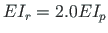
Example 3.1 Problem Statement. Depicted in Fig. 3.1 is a two-span frame. The height of the frame $h = 4{\,}\mathrm{m}$ , the two spans are of the same length: $l = 6{\,}\mathrm{m}$ . 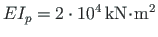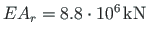Let us assume that the flexural rigidity of the column $EI_{p} = 2\cdot10^{4} {\,}\mathrm{kN}\hspace*{-2pt}\cdot\hspace*{-2pt}\mathrm{m}^{2}$ and that of the beam $EI_{r} = 2.0EI_{p}$ , the axial rigidity of the column $EA_{p} = 4.6\cdot10^{6}{\,}\mathrm{kN}$ and that of the beam $EA_{r} = 8.8\cdot10^{6}{\,}\mathrm{kN}$ , and the shear rigidity of the column 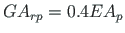$GA_{rp} = 0.4EA_{p}$ and that of the beam $GA_{rr} = 0.4EA_{r}$ . A uniform load for the first span $q = 8{\,}\mathrm{kN/m}$ . The central column is loaded with a concentrated load $F = 10{\,}\mathrm{kN}$ .

**Figure 3.1:** The two-span frame
$\includegraphics[width=100mm]{joonised/raamn2esREM.eps}$

We wish to compute the displacements, reactions, internal forces, and draw the axial force, shear force and bending moment diagrams.

Problem Solving. To solve the problem, we use the EST method. The solving procedure includes the following.

Data input: the number of frame nodes, elements, support reactions; element properties, elements loads in local coordinates, node forces in global coordinates, nodal coordinates, topology and hinges, restrictions on support displacements.

$\displaystyle \mathbf{spA}{\cdot}\mathbf{Z} = \mathbf{B}$ (3.1)
Assembling and solving the boundary problem equations (2.1) and (3.1) (prepared and solved by the program). To implement this aim, the program
1. inserts the basic equations of a frame into the equation system,
2. adds the compatibility equations of the displacements at nodes to the equation system,
3. adds the joint equilibrium equations,
4. adds the side conditions (hinges),
5. adds the restrictions on support displacements,
6. solves the compiled system of sparse equations,
7. produces an output: initial parameter vectors for element displacements and forces; support reactions.
Output: element displacements and forces determined by the transfer matrix.

1. Input data for the GNU Octave program spESTframeLaheWFI.m are shown in excerpts from the program: element and nodal loads - excerpt 3.1; nodal coordinates - excerpt 3.2; element properties, topology and hinges - excerpt 3.3.

Program excerpt 3.1 ( spESTframeLaheWFI.m )

 Number_of_frame_nodes=6 
 Number_of_elements=5
 Number_of_support_reactions=8
 spNNK=12*Number_of_elements+Number_of_support_reactions;
 Number_of_unknowns=spNNK 
 Displacements and forces are calculated on parts ("Nmitmeks") of the element
 Nmitmeks=4
# --- Element properties ---

  
 EIp=20000 # kN/m^2
 EIr=40000 # kN/m^2
 EAp=4.6*10^6 
#EAp=4.6*10^15; 
 EAr=6.8*10^6
#EAr=6.8*10^15; 
 GAp=0.4*EAp 
 GAr=0.4*EAr

baasi0=EIp/4 # scaling multiplier for displacements # baasi0=1.0; #Element load in local coordinates # qz qx qA qL # Uniformly distributed load in local coordinate z and x directions LoadsqONelement=4; esQkoormus=zeros(LoadsqONelement,4,ElementideArv);

esQkoormus(1,1:4,1)=[0.0 0.0 0.0 4.0]; 
esQkoormus(1,1:4,2)=[8.0 0.0 0.0 6.0];
esQkoormus(1,1:4,3)=[0.0 0.0 0.0 4.0]; 
esQkoormus(1,1:4,4)=[0.0 0.0 0.0 6.0]; 
esQkoormus(1,1:4,5)=[0.0 0.0 0.0 4.0];

# # Point load in local coordinate z and x directions kN # Fz, Fx, aF (coordinate of the point of force application) LoadsF_on_Element=5; esFjoud=zeros(LoadsF_on_Element,2,ElementideArv);

esFjoud(1,1:3,1)=[0.0 0.0 4.0];
esFjoud(1,1:3,2)=[0.0 0.0 6.0]; 
esFjoud(1,1:3,3)=[10.0 0.0 2.0];   
esFjoud(1,1:3,4)=[0.0 0.0 6.0];
esFjoud(1,1:3,5)=[0.0 0.0 4.0];

# #Node forces in global coordinates # sSolmF(forces,1,nodes); forces=[Fx; Fz; My] sSolmF = zeros(3,1,SolmedeArv);

#sSolmF(:,1,1)= 0.0
#sSolmF(:,1,2)= 0.0
#sSolmF(:,1,3)= 0.0
#sSolmF(:,1,4)= 0.0
#sSolmF(:,1,5)= 0.0
#sSolmF(:,1,6)= 0.0

# #s1F(1,1,1)=0.0; # force Fz #s1F(2,1,1)=0.0; # force Fz #s1F(3,1,1)=0.0; # force My # Support shift - tSiire# # Support shift is multiplied by scaling multiplier tSiire = zeros(3,1,SolmedeArv);

#tSiire(:,1,1)= 0.0
#tSiire(2,1,1)= 0.01*baasi0
#tSiire(:,1,2)= 0.0
#tSiire(:,1,3)= 0.0
#tSiire(:,1,4)= 0.0
#tSiire(:,1,5)= 0.0

Program excerpt 3.2 (Support reactions of the spESTframeLaheWFI.m )
#========== # Nodal coordinates #========== krdn=[# x z 0.0 0.0; % node 1 0.0 -4.0; % node 2 6.0 0.0; % node 3 6.0 -4.0; % node 4 12.0 0.0; % node 5 12.0 -4.0]; % node 6 #========== # #========== # Restrictions on support displacements (on - 1, off - 0) # Support No u w fi #========== tsolm=[1 1 1 0; % node 1 3 1 1 1; % node 3 5 1 1 1]; % node 5 #==========

Program excerpt 3.3 ( spESTframeLaheWFI.m )
# ------------- Element properties, topology and hinges --------- elasts=[# Element properties # n2 - end of the element # n1 - beginning of the element # N, Q, M - hinges at the end of the element # N, Q, M - hinges at the beginning of the element # EIp EAp GAp 2 1 0 0 1 0 0 1; % element 1 EIr EAr GAr 4 2 0 0 0 0 0 1; % element 2 EIp EAp GAp 4 3 0 0 0 0 0 0; % element 3 EIr EAr GAr 6 4 0 0 1 0 0 0; % element 4 EIp EAp GAp 5 6 0 0 0 0 0 1]; % element 5 # 1 - hinge 'true' (axial, shear, moment hinges) #

2. Assembling and solving the boundary problem equations (3.1), carried out by the function LaheFrameDFIm(baasi0,Ntoerkts,esQkoormus,esFjoud, sSolmF,tsolm,tSiire, krdn,selem). The program has numbered the displacements at element ends of the frame as shown in Fig. 3.2 and forces at element ends of the frame as shown in Fig. 3.3.

Figure 3.2: Numeration of displacements at frame element ends

$\includegraphics[width=100mm]{joonised/raam3esREMSiir.eps}$

Figure 3.3: Numeration of forces at frame element ends

$\includegraphics[width=100mm]{joonised/raam3esREMStoe.eps}$

The unscaled initial parameter vectors of the elements are shown in excerpt 3.1 from the computing diary.

Computing diary excerpt 3.1 ( spESTframeLaheWFI.m )
-------- Scaling multiplier for displacements = 1/baasi0 -------- ============================================================================ Unscaled initial parameter vector Element u w fi N Q M No ---------------------------------------------------------------------------- 1 -0.000e+00 0.000e+00 8.881e-06 20.301 0.000 0.000 2 -3.552e-05 1.765e-05 -1.247e-03 0.000 -20.301 0.000 3 -0.000e+00 0.000e+00 0.000e+00 29.980 -10.033 11.622 4 -3.552e-05 2.607e-05 6.889e-04 -0.033 -2.281 13.684 5 -1.983e-06 3.549e-05 1.331e-05 -2.281 0.033 0.000 ----------------------------------------------------------------------------

The support reactions of the frame in global coordinates are shown in excerpt 3.2 from the computing diary.

Computing diary excerpt 3.2 ( spESTframeLaheWFI.m )
Support reactions begin from row X: 61 =========================================== No X Node Cx <=> 1 Cz <=> 2 Cy <=> 3 ------------------------------------------- 61 -0.000000e+00 1 1 62 -2.030089e+01 1 2 63 -1.003327e+01 3 1 64 -2.997974e+01 3 2 65 +1.162223e+01 3 3 66 +3.327478e-02 5 1 67 +2.280630e+00 5 2 68 -1.330991e-01 5 3 -------------------------------------------

3. Output: the element displacements and forces determined by the transfer matrix.

Computing diary excerpt 3.3 ( spESTframeLaheWFI.m )
#================================================================================= Element displacements and forces determined by transfer matrix #================================================================================= Displacements and forces of element no 1 of length 4.000 m The element is divided into 4 parts displacement u - 0.00000e+00 -4.41324e-06 -8.82647e-06 -1.32397e-05 -1.76529e-05 displacement w - 0.00000e+00 -8.88062e-06 -1.77612e-05 -2.66418e-05 -3.55225e-05 rotation fi - 8.88062e-06 8.88062e-06 8.88062e-06 8.88062e-06 8.88062e-06 normal force N - -20.30089 -20.30089 -20.30089 -20.30089 -20.30089 shear force Q - 0.00000 0.00000 0.00000 0.00000 0.00000 moment force M - 0.00000 0.00000 0.00000 0.00000 0.00000 ---------------------------------------------------------------------------- Displacements and forces of element no 2 of length 6.000 m The element is divided into 4 parts displacement u - -3.55225e-05 -3.55225e-05 -3.55225e-05 -3.55225e-05 -3.55225e-05 displacement w - 1.76529e-05 2.12539e-01 3.37647e+00 1.70839e+01 5.39892e+01 rotation fi - -1.24654e-03 -5.63176e-01 -4.49896e+00 -1.51836e+01 -3.59921e+01 normal force N - 0.00000 0.00000 0.00000 0.00000 0.00000 shear force Q - 20.30089 8.30089 -3.69911 -15.69911 -27.69911 moment force M - 0.00000 21.45134 24.90267 10.35401 -22.19465 ---------------------------------------------------------------------------- Displacements and forces of element no 3 of length 4.000 m The element is divided into 4 parts displacement u - 0.00000e+00 -6.51733e-06 -1.30347e-05 -1.95520e-05 -2.60693e-05 displacement w - 0.00000e+00 2.06945e-04 4.93338e-04 4.17024e-01 3.33263e+00 rotation fi - 0.00000e+00 -3.30279e-04 -1.58895e-04 -1.24949e+00 -4.99831e+00 normal force N - -29.97974 -29.97974 -29.97974 -29.97974 -29.97974 shear force Q - 10.03327 10.03327 0.03327 0.03327 0.03327 moment force M - -11.62223 -1.58895 8.44432 8.47760 8.51087 ---------------------------------------------------------------------------- Displacements and forces of element no 4 of length 6.000 m The element is divided into 4 parts displacement u - -3.55225e-05 -3.55151e-05 -3.55078e-05 -3.55004e-05 -3.54931e-05 displacement w - 2.60693e-05 -6.54442e-04 -7.57670e-04 -4.76041e-04 -1.98316e-06 rotation fi - 6.88865e-04 2.39865e-04 -8.08482e-05 -2.73276e-04 -3.37419e-04 normal force N - 0.03327 0.03327 0.03327 0.03327 0.03327 shear force Q - 2.28063 2.28063 2.28063 2.28063 2.28063 moment force M - -13.68378 -10.26284 -6.84189 -3.42095 0.00000 ---------------------------------------------------------------------------- Displacements and forces of element no 5 of length 4.000 m The element is divided into 4 parts displacement u - -1.98316e-06 -1.48737e-06 -9.91578e-07 -4.95789e-07 4.23516e-22 displacement w - 3.54931e-05 2.24605e-05 1.10916e-05 3.05019e-06 3.38813e-21 rotation fi - 1.33099e-05 1.24780e-05 9.98244e-06 5.82309e-06 -1.69407e-21 normal force N - 2.28063 2.28063 2.28063 2.28063 2.28063 shear force Q - -0.03327 -0.03327 -0.03327 -0.03327 -0.03327 moment force M - 0.00000 -0.03327 -0.06655 -0.09982 -0.13310 ----------------------------------------------------------------------------

Figure 3.4: Bending moment diagram $\qquad$ of the two-span frame

$\begin{picture}(80,38.8) \centering \includegraphics[width=80mm]{joonised/ajouOctave04est.eps} \end{picture}$


         In Figs. 3.4 and 3.5, the values in brackets are determined with the axial stiffness $EA_{p} = 4.6\cdot 10^{15}{\,}\mathrm{kN}$ (with negligible axial deformations; the values coincide with these found with the force method, see [Lah12] Fig. 9.13 on p. 232).
The values without brackets are calculated with the axial stiffness $EA_{p} = 4.6\cdot 10^{6}{\,}\mathrm{kN}$ .

The shear force Q and the axial force N diagrams of the two-span frame are shown in Fig. 3.5.

Figure 3.5: Diagrams of the axial force N and shear force Q of the two-span frame

$\includegraphics[width=0.98\textwidth]{joonised/ajou3QjaNest.eps}$

Figure 3.6: Boundary forces of the two-span frame

$\includegraphics[width=80mm]{joonised/ajou3ToedEst.eps}$

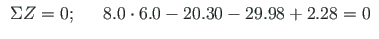
Testing a static equilibrium for the frame
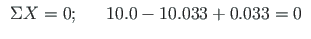
Consider a static equilibrium of the frame shown in Fig. 3.6. When projecting the forces onto the X-axis,

$\displaystyle \begin{array}{ccl} \Sigma X = 0; & & 10.0 - 10.033 + 0.033 = 0 \end{array}$ (3.2)

and onto the Z-axis,

$\displaystyle \begin{array}{ccl} \Sigma Z = 0; & & 8.0\cdot 6.0 - 20.30 - 29.98 + 2.28 = 0 \end{array}$ (3.3)

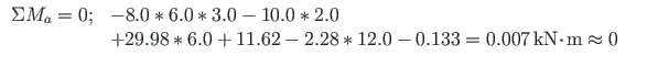
We now write equation (3.4) of the sum of the moments and the moments of the forces acting about point a shown in Fig. 3.6:

$\displaystyle \begin{array}{ll} \Sigma M_{a} = 0; &- 8.0\cdot 6.0\cdot 3.0 - 10... ...thrm{kN}\hspace*{-2pt}\cdot\hspace*{-2pt}\mathrm{m} \approx 0 \quad \end{array}$ (3.4)

The calculations with equations (3.2), (3.3), and (3.4) have verified the static equilibrium of the frame.
In Fig. 3.7, the elements, and in Fig. 3.8, the sparsity pattern of matrix spA of the two-span frame are shown.

Figure 3.7: Elements of the two-span frame

$\includegraphics[width=0.82\textwidth]{joonised/RaamESTen.eps}$

Figure 3.8: Sparsity pattern of matrix spA of the two-span frame

$\includegraphics[width=0.77\textwidth]{joonised/spESTframe_sparse_en.eps}$