4.1 Illustrative frame problem

Example 4.1 Problem Statement. Figure 4.1 shows a frame with the dimensions as follows: height of the column $h = 4{\,}\mathrm{m}$ , height of the frame $5{\,}\mathrm{m}$ , span length $l = 8{\,}\mathrm{m}$ . The rafter 2-3 is loaded with a vertical uniform load $q = 2.0{\,}\mathrm{kN/m}$ , the rafter 3-4 is loaded with a vertical concentrated load $F_{1} = 3.0{\,}\mathrm{kN}$ , and the joint 2 is subjected to a horizontal load $F_{2}= 1.0{\,}\mathrm{kN}$ .

**Figure 4.1:** The three-hinged frame EST1
$\includegraphics[width=112mm]{joonised/raamNaEST1.eps}$

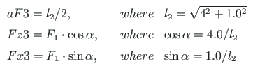
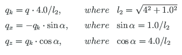
Consider the load transformation from the global system to the local one shown in Figs. 4.1 b and 4.2. The force $F_{1}$ is transformed to , :

$\displaystyle \begin{array}{lll} aF3=l_{2}/2, &\quad where & l_{2} = \sqrt{4^{2... ... Fx3 = F_{1}\cdot\sin\alpha, &\quad where & \sin\alpha = 1.0/l_{2} \end{array}$

(4.1)

The vertical load is transformed to $q_{x}$ , $q_{z}$ :

$\displaystyle \begin{array}{lll} q_{k} = q\cdot 4.0/l_{2}, &\quad where & l_{2}... ...q_{z} = q_{k}\cdot\cos\alpha, &\quad where & \cos\alpha = 4.0/l_{2} \end{array}$

(4.2)

**Figure 4.2:** Numeration of displacements and forces of the frame EST1
$\includegraphics[width=85mm]{joonised/raamNaEST1numbr.eps}$

We wish to compute the reactions and internal forces, and draw the axial force, shear force and bending moment diagrams.

Problem Solving. To solve the problem, we use the EST method. The solving procedure includes the following.

Data input: the number of frame nodes, elements, support reactions; element loads in local coordinates, node forces in global coordinates, nodal coordinates, topology and hinges.

$\displaystyle \mathbf{spA}{\cdot}\mathbf{Z} = \mathbf{B}$ (4.3)
Assembling and solving the boundary problem equations (4.3) (prepared and solved by the program):
1. writing the basic equations of a frame in transfer matrix form,
2. adding the joint equilibrium equations,
3. adding the side conditions (hinges),
4. solving the system of sparse equations,
5. producing an output: initial parameter vectors for element forces; support reactions.
Output: element forces determined by the transfer matrix.

1. Input data for the GNU Octave program spESTframe3hingeLaheNQM.m are given in excerpts from the program: element and nodal loads - excerpt 4.1; nodal coordinates - excerpt 4.2; element properties, topology and hinges - excerpt 4.3.

Program excerpt 4.1 ( spESTframe3hingeLaheNQM.m )

 Number_of_frame_nodes=5
 Number_of_elements=4
 Number_of_support_reactions=4
 spNNK=6*Number_of_elements+Number_of_support_reactions;
 Number_of_unknowns=spNNK 
 Forces are calculated on parts ("Nmitmeks") of the element  
 Nmitmeks=4
 Lp=8.0; # graphics axes
# --- Element loads ---

  
 F1=3.0;
L2x=sqrt(4.0^2+1.0^2);  # length of 
                          the element
Lpunkt=L2x/2;
F2=1.0;
q=2.0;
sinA2=1.0/L2x;
cosA2=4.0/L2x;
qk=2.0*4.0/L2x; 
#esQkoormus  qz2 qx2 0.0 L2x
qz2=qk*cosA2;  # projection onto z-axis
qx2=-qk*sinA2; # projection onto x-axis
#
#esFjoud Fz3 Fx3 aF3
Fz3=F1*cosA2; # projection onto z-axis
Fx3=F1*sinA2; # projection onto x-axis
aF3=L2x/2;
# ---- load variants -----
load_variant=1
#load_variant=2
#load_variant=3

switch (koormusvariant) case{1} disp(' Load variant 1 ')
#Element load in local coordinates # qz qx qA qL # Uniformly distributed load in local coordinate z and x directions LoadsqONelement=4; esQkoormus=zeros(LoadsqONelement,4,ElementideArv);

esQkoormus(1,1:4,1)=[0.0 0.0 0.0 4.0];
esQkoormus(1,1:4,2)=[qz2 qx2 0.0 L2x];
esQkoormus(1,1:4,3)=[0.0 0.0 0.0 L2x];
esQkoormus(1,1:4,4)=[0.0 0.0 0.0 4.0];

# Point load in local coordinate z and x directions kN # Fz, Fx, aF (coordinate of the point of force application) LoadsF_on_Element=5; esFjoud=zeros(LoadsF_on_Element,2,ElementideArv);

esFjoud(1,1:3,1)=[0.0 0.0 0.0];
esFjoud(1,1:3,2)=[0.0 0.0 0.0];  
esFjoud(1,1:3,3)=[Fz3 Fx3 aF3]; 
esFjoud(1,1:3,4)=[0.0 0.0 0.0];
esFjoud(1,1:3,5)=[0.0 0.0 0.0];

#Node forces in global coordinates # sSolmF(forces,1,nodes); forces=[Fx; Fz; My] sSolmF = zeros(3,1,SolmedeArv);

#sSolmF(:,1,1)= 0.0
sSolmF(1,1,2)= F2;
#sSolmF(:,1,3)= 0.0
#sSolmF(:,1,4)= 0.0
#sSolmF(:,1,5)= 0.0

#s1F(1,1,1)=0.0; # force Fz #s1F(2,1,1)=0.0; # force Fz #s1F(3,1,1)=0.0; # force My
case{2} disp(' Load variant 2 ') case{3} disp(' Load variant 3 ') # otherwise disp(' No load variant cases ') endswitch

Program excerpt 4.2 ( spESTframe3hingeLaheNQM.m )
#========== # Nodal coordinates #========== krdn=[# x z 0.0 0.0; # node 1 0.0 -4.0; # node 2 4.0 -5.0; # node 3 8.0 -4.0; # node 4 8.0 0.0]; # node 5 #========== # Restrictions on support displacements (on - 1, off - 0) # Support No u w fi #========== tsolm=[1 1 1 0; % node 1 5 1 1 0]; % node 5 #==========

Program excerpt 4.3 ( spESTframe3hingeLaheNQM.m )
# ------------- Element properties, topology and hinges --------- elasts=[# Element # n2 - end of the element # n1 - beginning of the element # N, Q, M - hinges at the end of the element # N, Q, M - hinges at the beginning of the element 2 1 0 0 0 0 0 1; % element 1 3 2 0 0 1 0 0 0; % element 2 4 3 0 0 0 0 0 1; % element 3 5 4 0 0 1 0 0 0]; % element 4 # 1 - hinge 'true' (axial, shear, moment hinges) #

2. Assembling and solving the boundary problem equations (4.3), carried out by the function LaheFrame3hingeNQM(baasi0,Ntoerkts,esQkoormus,esFjoud,sSolmF,tsolm, tSiire,krdn,selem). The program has numbered the forces at element ends of the frame as shown in Fig. 4.2.
The initial parameter vectors of the elements are given in excerpt 4.1 from the computing diary.

Computing diary excerpt 4.1 ( spESTframe3hingeLaheNQM.m )
=========================================== Initial parameter vector Element No N Q M ------------------------------------------- 1 6.250 1.600 0.000 2 4.038 -5.433 6.400 3 2.947 1.067 0.000 4 4.750 -2.600 10.400 -------------------------------------------

The support reactions of the frame in global coordinates are shown in excerpt 4.2 from the computing diary.

Computing diary excerpt 4.2 ( spESTframe3hingeLaheNQM.m )

Support reactions begin from X row: 25 =========================================== No X Node Cx <=> 1 Cz <=> 2 Cy <=> 3 ------------------------------------------- 25 +1.600000e+00 1 1 26 -6.250000e+00 1 2 27 -2.600000e+00 5 1 28 -4.750000e+00 5 2 --------------------------------------------

3. Output: the forces determined by the transfer matrix are shown in excerpt 4.3 from the computing diary.

Computing diary excerpt 4.3 ( spESTframe3hingeLaheNQM.m )

#======================================================================= Element forces determined by transfer matrix #======================================================================= Forces of element no 1 of length 4.000 m The element is divided into 4 parts normal force N - -6.250 -6.250 -6.250 -6.250 -6.250 shear force Q - -1.600 -1.600 -1.600 -1.600 -1.600 moment force M - 0.000 -1.600 -3.200 -4.800 -6.400 ------------------------------------------------------------------------ Forces of element no 2 of length 4.123 m The element is divided into 4 parts normal force N - -4.038 -3.553 -3.068 -2.583 -2.098 shear force Q - 5.433 3.493 1.552 -0.388 -2.328 moment force M - -6.400 -1.800 0.800 1.400 -0.000 ------------------------------------------------------------------------ Forces of element no 3 of length 4.123 m The element is divided into 4 parts normal force N - -2.947 -2.947 -3.674 -3.674 -3.674 shear force Q - -1.067 -1.067 -3.978 -3.978 -3.978 moment force M - 0.000 -1.100 -2.200 -6.300 -10.400 ------------------------------------------------------------------------ Forces of element no 4 of length 4.000 m The element is divided into 4 parts normal force N - -4.750 -4.750 -4.750 -4.750 -4.750 shear force Q - 2.600 2.600 2.600 2.600 2.600 moment force M - -10.400 -7.800 -5.200 -2.600 -0.000 ------------------------------------------------------------------------

Testing a static equilibrium for the frame
Consider next a static equilibrium of the frame shown in Fig. 4.3. We project the forces onto the X, Z axes and determine the sum of the moments of the forces acting about point 1. The sums of the forces and moments are:

$\displaystyle \begin{array}{lcl} \Sigma X = 0; & & 1.6 + 1.0 - 2.6 = 0 \\ \Sig... ... \Sigma M_{1} = 0; & & 4.75\cdot 8 - 1\cdot 4 - 2\cdot 4\cdot 2 = 0 \end{array}$ (4.4)

The calculations shown in equations (4.4) have verified the static equilibrium of the frame.

Figure 4.3: Support reactions of the frame EST1

$\includegraphics[width=90mm]{joonised/raamNaEST1STR.eps}$

The bending moment M, shear force Q and axial force N diagrams of the statically determined three-hinged frame EST1 are shown in Fig. 4.4.

Figure 4.4: Internal forces diagrams of the three-hinged frame EST1
             $\includegraphics[width=73mm]{joonised/raamNa1eMe.eps}$
                  [Bending moment diagram]

$\includegraphics[width=69mm]{joonised/raamNa2eQe.eps}$
          [Shear force Q diagram]


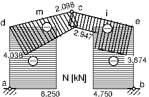
           [Axial force N diagram]

The elements of the frame are depicted in Fig. 4.5 and the sparsity pattern of matrix spA of the frame is shown in Fig. 4.6.
The displacements can be computed with the GNU Octave program spESTframe3hingeLaheWFI.m.

Figure 4.5: Elements of the three-hinged frame EST1

$\includegraphics[width=0.75\textwidth]{joonised/RaamEST3liigendigaE.eps}$

Figure 4.6: Sparsity pattern of matrix spA of the three-hinged frame EST1

$\includegraphics[width=0.75\textwidth]{joonised/RaamEST3liigendiga_h6remE.eps}$

$\includegraphics[width=73mm]{joonised/raamNa1eMe.eps}$ [Bending moment diagram]
$\includegraphics[width=69mm]{joonised/raamNa2eQe.eps}$ [Shear force Q diagram]	[Axial force N diagram]